Uniform random numbers? We can do better…

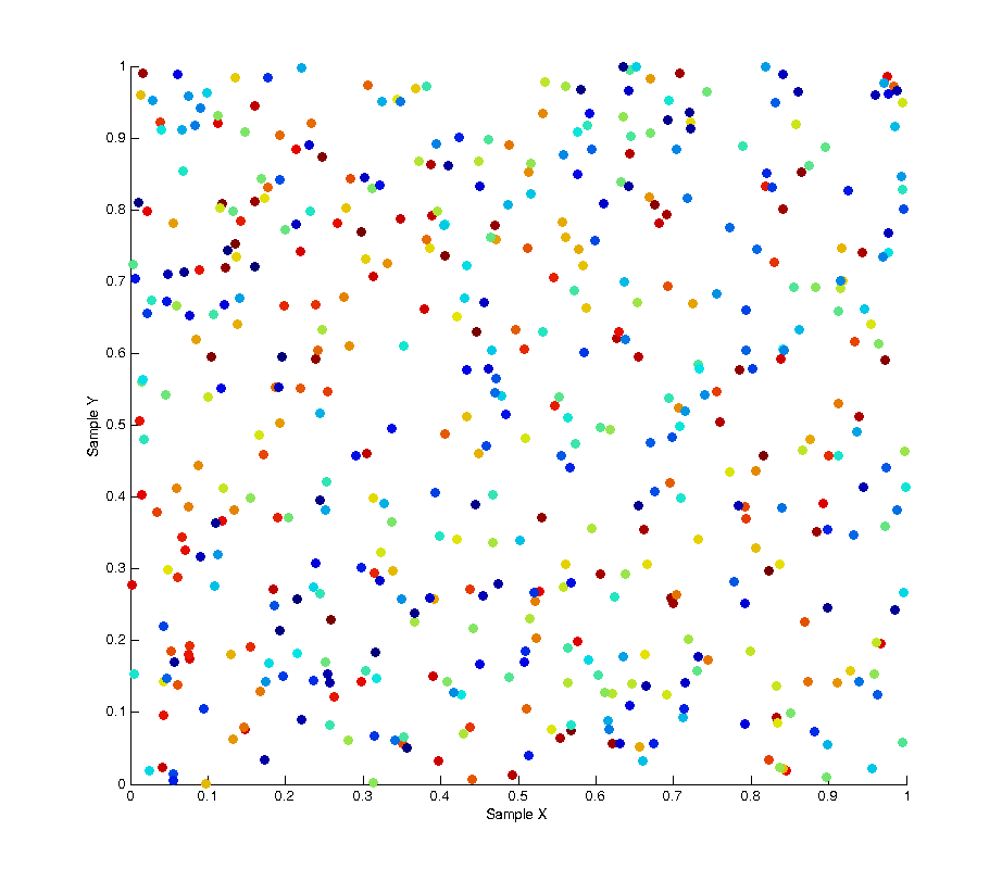
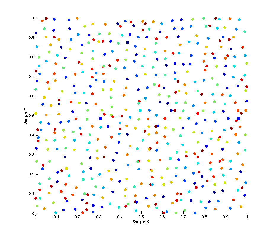
In monte carlo rendering we need random numbers. Like… a lot of random numbers. In fact if you count every call to the random functions in a single render it can easily surpass a several million numbers. Not only do we need lots of numbers, but we tend to need ones which have certain desirable properties such as proper uniformity without accidental bunching. To explain the problem being addressed, the image below shows 500 “uniform” random samples over a [0.0, 1.0] square, where the colour of each sample refers to its order throughout the sampling (blue -> red). As you can see the result of this leads to bunching and poor distribution over the entire sample space with some areas being under-sampled and some areas over-sampled. In the use case of image anti-aliasing this can lead to duplication of expensive computations on similar sub-pixels while other areas of the pixel space get left un-sampled.

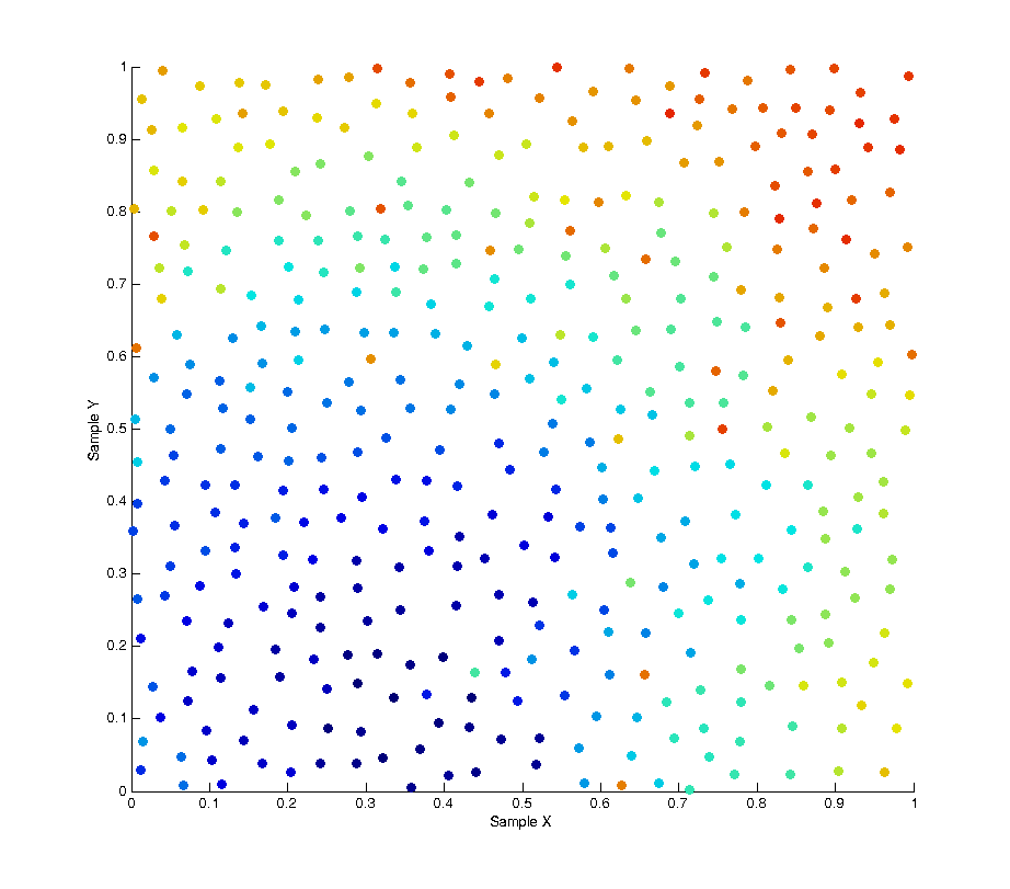
One possible solution to this is Poisson Disk Sampling which aims to solve the problem of sample distribution by creating a whole batch of samples at once where each sample is at least a minimum distance from any other sample. Because samples have to be generated in batches this leads to a high correlation between samples due to the fact that after an initial “seed” sample is chosen all subsequent ones are the product of growing outwards from this seed. As can be seen in the image below Poisson sampling gives a nice, lamina, distribution of samples over the sample space. The below image is the product of 500 samples of Poisson sampling with a minimum distance of 0.05. At this distance setting the sampling tends to generate samples in batches of approximately 400 samples, whenever the list of batched samples is depleted a new batch is produced.

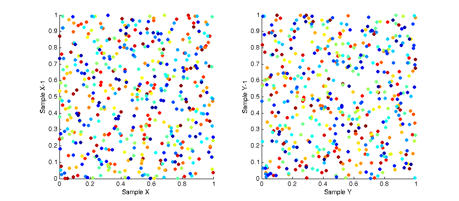
While the overall distribution of samples appears lamina, the intermediate distribution at any discrete interval throughout the sampling is not. This is due to the fact samples are “grown” in batches. The image below shows the affect of this correlation by plotting the X and Y values of each sample with respect to the X and Y values of the previous samples. As you can see a strong pattern emerges across each axis.

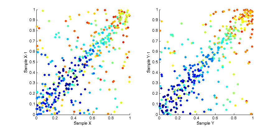
To remove this bias we can use a technique called a “random pop” to select elements from within each batch uniformly rather than in sequence. At each sample we select a random element from the batch, then copy the last element of the list into that spot and pop the last element from the list before returning the random element we selected. The result of this solution is that at any point within a given batch of samples the distribution of samples is uncorrelated and unbiased. This is shown in the image below, as you can see the colour of each sample is now randomly distributed.

By plotting the correlation between samples again we can also see there is no pattern across the whole set of samples.

Tags Poisson, Sampling, Uniform