Yesterday I stumbled upon a lesser known and far superior method for mapping points from a square to a disk. The common approach which is presented to you after a quick google for Draw Random Samples on a Disk is the clean and simple mapping from Cartesian to Polar coordinates; i.e.
Given a disk centered origin (0,0) with radius r
// Draw two uniform random numbers in the range [0,1)
R1 = RAND(0,1);
R2 = RAND(0,1);

// Map these values to polar space (phi,radius)
phi = R1 * 2PI;
radius = R2 * r;

// Map (phi,radius) in polar space to (x,y) in Cartesian space
x = cos(phi) * radius;
y = sin(phi) * radius;
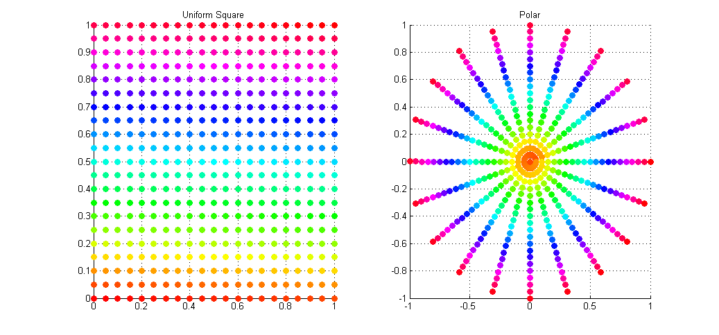
The result of this sampling on a regular grid of samples is shown in the image below. The left plot shows the input points as simple ordered pairs in the range [0,1)^2, while the right plot shows these same points (colour for colour) mapped onto a unit disk using Polar mapping as described above.
As you can see the mapping is not ideal with many points being over-sampled at the poles (I wonder why they call is Polar coordinates), and with areas towards the radius left under-sampled. What we would actually like is a disk sampling strategy that keeps the uniformity seen in the square distribution while mapping the points onto the disk.
Enter, Concentric Disk Sampling. This paper by Shirley & Chiu presents the idea for warping the unit square into that of a unit circle. Their method is nice but it contains a lot of nested branching for determining which quadrant the current point lays within. Shirley mentions an improved variant of this mapping on his blog, accredited to Dave Cline. Cline’s method only uses one if-else branch and is simpler to implement.
Again, given a disk centered origin (0,0) with radius r
// Draw two uniform random numbers in the range [0,1)
R1 = RAND(0,1);
R2 = RAND(0,1);

// Avoid a potential divide by zero
if (R1 == 0 && R2 == 0) {
    x = 0; y = 0;
    return;
}

// Initial mapping
phi = 0; radius = r;
a = (2 * R1) - 1;
b = (2 * R2) - 1;

// Uses squares instead of absolute values
if ((a*a) > (b*b)) {
    // Top half
    radius  *= a;
    phi = (pi/4) * (b/a);
}
else {
    // Bottom half
    radius *= b;
    phi = (pi/2) - ((pi/4) * (a/b));
}

// Map the distorted Polar coordinates (phi,radius)
// into the Cartesian (x,y) space
x = cos(phi) * radius;
y = sin(phi) * radius;
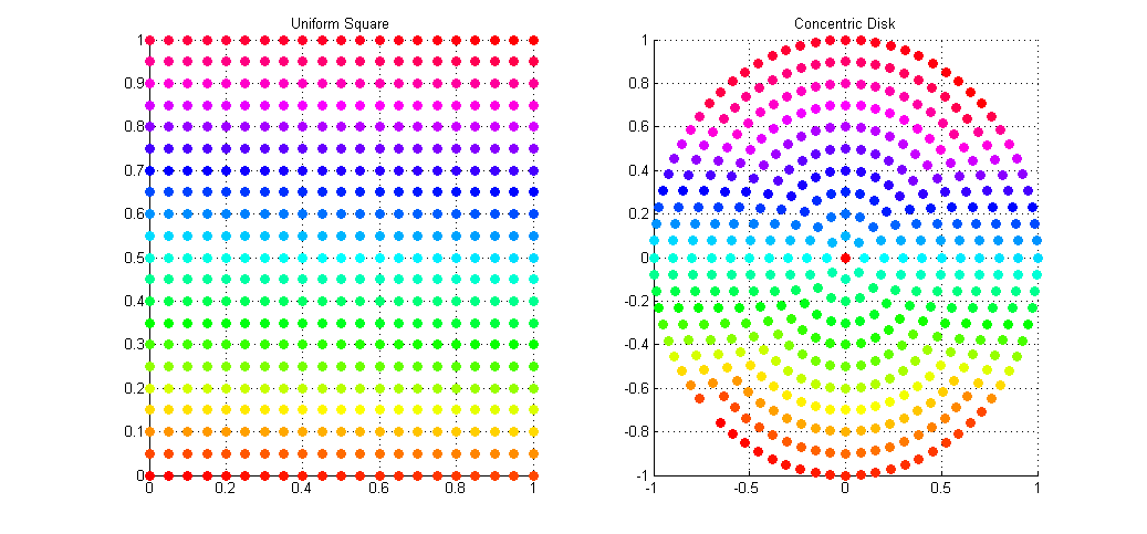
This gives a uniform distribution of samples over the disk in Cartesian space. The result of the mapping applied to the same set of uniform square samples is shown above. Notice how we now get full coverage of the disk using just as many samples, and that each point has (relatively) equal distance to all of it’s neighbors, meaning no bunching at the poles, and no under-sampling at the fringe.
I’ve applied this sampling technique to my Path Tracer as a means of sampling the aperture of the virtual point camera when computing depth of field. Convergence to the true out-of-focus light distribution is now much faster and more accurate than it was with Polar sampling which, due to bunching at the poles, cause a disproportionate number of rays to be fired along trajectories very close to the true ray.
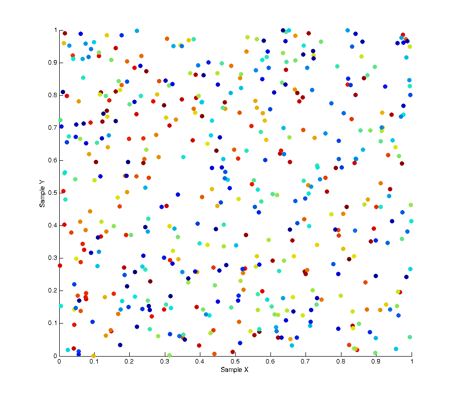
In monte carlo rendering we need random numbers. Like… a lot of random numbers. In fact if you count every call to the random functions in a single render it can easily surpass a several million numbers. Not only do we need lots of numbers, but we tend to need ones which have certain desirable properties such as proper uniformity without accidental bunching. To explain the problem being addressed, the image below shows 500 “uniform” random samples over a [0.0, 1.0] square, where the colour of each sample refers to its order throughout the sampling (blue -> red). As you can see the result of this leads to bunching and poor distribution over the entire sample space with some areas being under-sampled and some areas over-sampled. In the use case of image anti-aliasing this can lead to duplication of expensive computations on similar sub-pixels while other areas of the pixel space get left un-sampled.
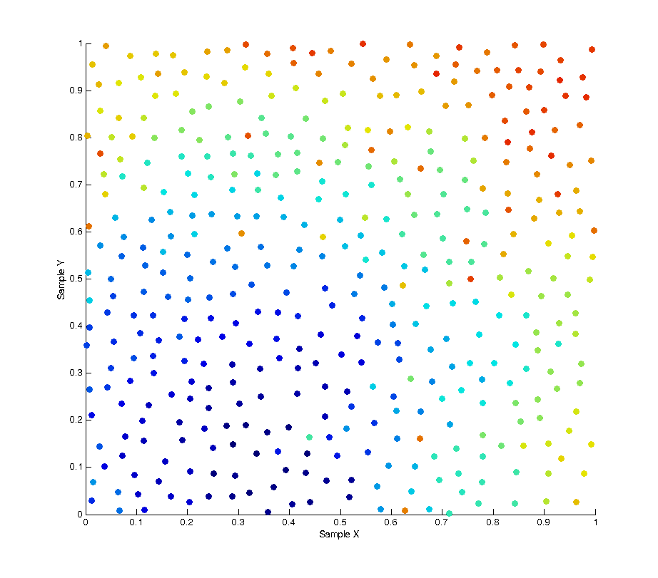
One possible solution to this is Poisson Disk Sampling which aims to solve the problem of sample distribution by creating a whole batch of samples at once where each sample is at least a minimum distance from any other sample. Because samples have to be generated in batches this leads to a high correlation between samples due to the fact that after an initial “seed” sample is chosen all subsequent ones are the product of growing outwards from this seed. As can be seen in the image below Poisson sampling gives a nice, lamina, distribution of samples over the sample space. The below image is the product of 500 samples of Poisson sampling with a minimum distance of 0.05. At this distance setting the sampling tends to generate samples in batches of approximately 400 samples, whenever the list of batched samples is depleted a new batch is produced.
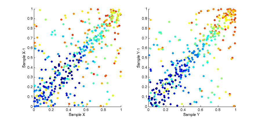
While the overall distribution of samples appears lamina, the intermediate distribution at any discrete interval throughout the sampling is not. This is due to the fact samples are “grown” in batches. The image below shows the affect of this correlation by plotting the X and Y values of each sample with respect to the X and Y values of the previous samples. As you can see a strong pattern emerges across each axis.
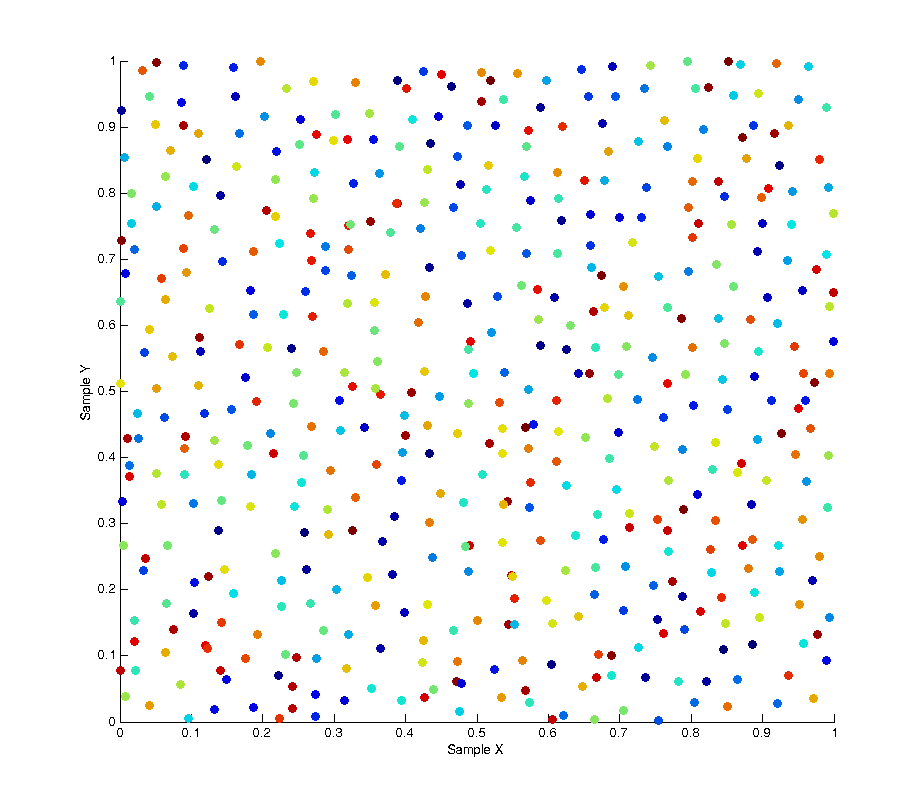
To remove this bias we can use a technique called a “random pop” to select elements from within each batch uniformly rather than in sequence. At each sample we select a random element from the batch, then copy the last element of the list into that spot and pop the last element from the list before returning the random element we selected. The result of this solution is that at any point within a given batch of samples the distribution of samples is uncorrelated and unbiased. This is shown in the image below, as you can see the colour of each sample is now randomly distributed.
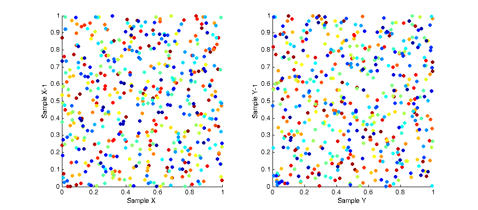
By plotting the correlation between samples again we can also see there is no pattern across the whole set of samples.
Pressing onwards with research after a short break to play with the Xeon Phi rack, I’ve been working on visualizations for Monte Carlo Simulations.
My aim is to have a clean and concise means of displaying (and therefore being able to infer relationships from) the data of higher dimensional probability distributions. The video below shows one such visualization where a 2D Gaussian PDF has been simulated using Hamiltonian Dynamics.
Hamiltonian Dynamics Monte Carlo
The two 3D meshes represent the reconstructed sample volume as a 2D histogram of values rescaled to the original function. The error between the reconstruction and the original curves is shown through the colour of the surface where hot spots denote areas of high error.
The mean sq error for the whole distribution is displayed in the top right on a logarithmic scale. An algorithm which converges in an ideal manner will graph it’s error as a straight line on the log scale.
The sample X and Y graphs in the bottom right allow us to visualize where the samples are being chosen as the simulation runs and infer about whether samples are being chosen independently of one another. The centre-bottom graph simply gives us a trajectory of samples over the course of the simulation. This allows us to additionally catch if an algorithm is prone to getting stuck in local maxima’s.
Metropolis Hastings Monte Carlo
The above video shows the same simulation run with a basic Metropolis Hastings algorithm. Here the proposal sample x and y attributes are chosen independently of one another, meaning this is not a Gibbs Sampler. Although I intend to implement one within the test framework for comparisons sake soon.
A key difference between the two simulations here is to note the Path Space Trajectory shown in the bottom-centre graph and how it relates to the Sample Dimension Space graphs shown on the middle & bottom-right. Hamiltonian Dynamics chooses sets of variables where the x and y elements are highly dependent on one another within a coordinate, yet almost entirely independent of other pairs of coordinates within the Path Space.
Metropolis Hastings on the other hand, chooses coordinate pairs entirely independently of one another, and values within each dimension of the Path Space that are highly dependent on one another. These characteristics of the Metropolis sampler are undesirable, which is why adding a dependency within coordinate pairs (Gibbs Sampling) helps to accelerate multi-dimensional Metropolis Samplers.
It’s been a couple of weeks since I stopped working directly on rendering and took some time to read up on a topic called Hamiltonian (Hybrid) Monte Carlo which is to be the main focus of my research for the foreseeable future.
Hamiltonian Monte Carlo comes from a physics term of the same genesis called Hamiltonian Dynamics. The general idea being that, like with a Lagrangian equation for a system, you find a way to model the energy of a system which allows you to estimate it at efficiently even when the system is highly dimensional. With a Lagrangian you aim to minimize the degrees of freedom to reduce computation, and similarly with a Hamiltonian you reduce the problem to a measure of the systems kinetic K(p) and potential U(x) energy. This allows you to describe the entire state of an arbitrarily dimensional system as the sum of these measures, i.e. H(x,p) = U(x) + K(p)
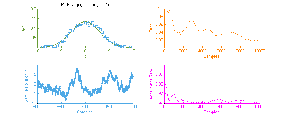
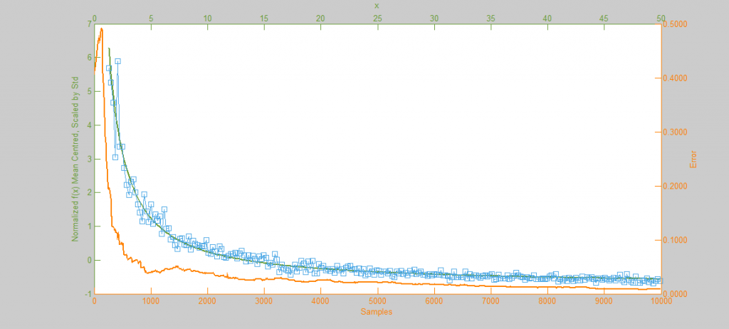
Above is our faithful companion, Metropolis Hastings Monte Carlo (MHMC), simulating a Normal distribution with mean “ and variance 3. The simulation was run for 10,000 samples yielding the shown results. Some things worth noting here are features such as the Error curve (Orange), which varies dramatically as simulation progresses. This is in-part due to the nature of the Random Walk which MHMC takes through the integration space which can be seen in the Blue graph to the bottom left. It is clear from the Blue graph that two states x and x' in the Makrov Chain are tightly dependent on one another.
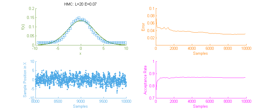
Next we see the same Normal distribution used above, estimated this time using Hamiltonian Monte Carlo (HMC) with trajectory length 20 and step size 0.07. To compare this to our previous simulation using MHMC several things become apparent. Firstly, The Error curve (Orange) seems to decay in a much more controlled and systematic manner. As opposed to the Error for MHMC which was erratic due to the nature of a Random Walk, here we see the benefit of making an informed choice as to where to place the next sample. From this we can hypothesise that a optimally tuned HMC simulation will in general reduce the error of the simulation with more samples consistently with little chance of introducing large, random, errors as with MHMC. Additionally in the sample placement graph (Blue) we see that the relationship between two states x and x' is far more abstracted, meaning two samples while being related and forming a valid Markov Chain will not reduce the accuracy of the simulation by treading on each others turf.
There is however, an issue with the above HMC simulation. Tuning. Unless properly tuned for the specific problem the Hyper-parameters for the Trajectory length L and Step size E will simply not work as intended and will yield poor results.
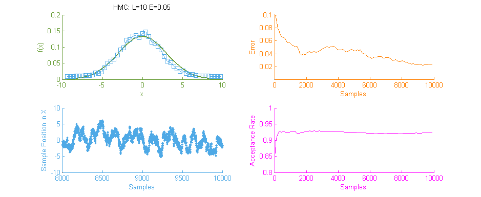
Above is a second run of the HMC simulation, this time with trajectory length 10 and step size 0.05. Because the length of the Leapfrog Trajectory was not sufficient to allow the system to move to an independent state we see the same banding of samples in the sample frequency graph (Blue) as we saw in the original Metropolis simulation. Additionally because of the dependent nature of the samples a similar pattern is seen in the Error curve (Orange) where the curve has large peaks where error was reintroduced to the system like with a Random Walk.
It is therefore vital to optimally tune HMC as the computation for each sample is an order of magnitude larger than with MHMC. Without proper tuning it’s much better to stick with the easier to tune MHMC.
So I’m still playing with graphs in Matlab… I shouldn’t complain, I know. I should be cherishing how laid back and relaxed the PhD experience is right now compared the where I’ll be a couple of years from now.
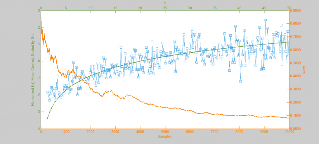
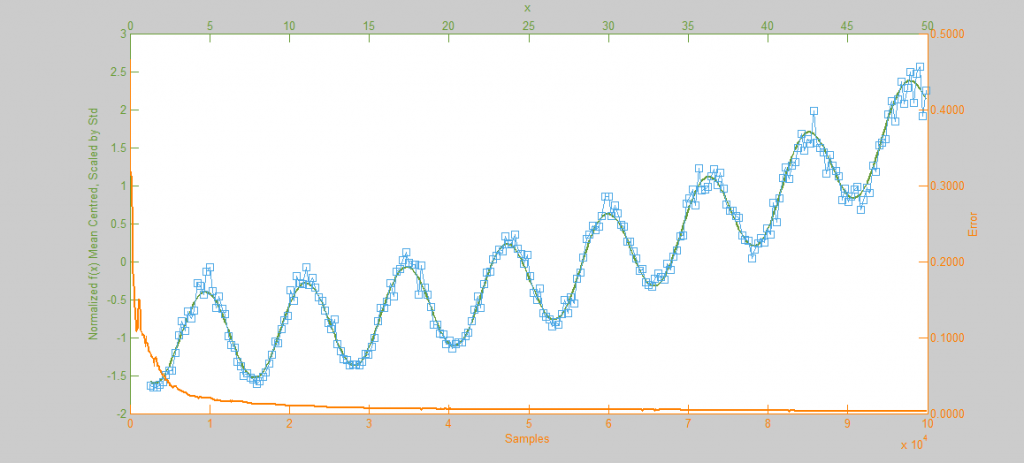
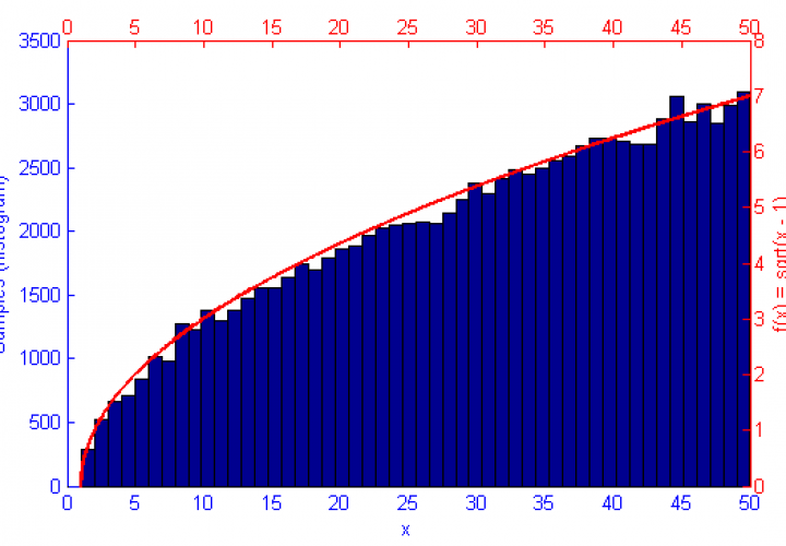
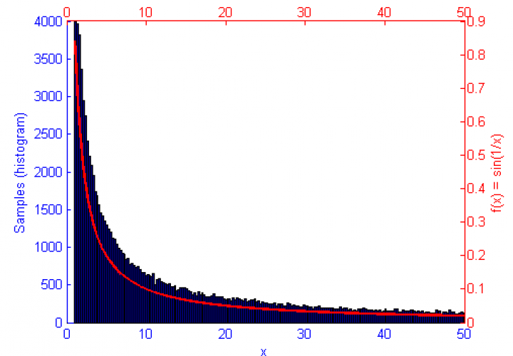
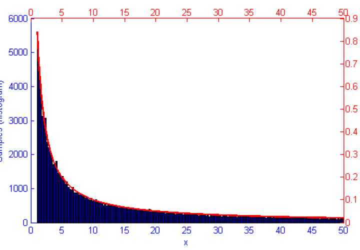
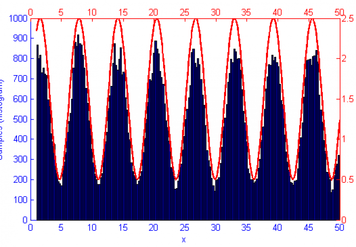
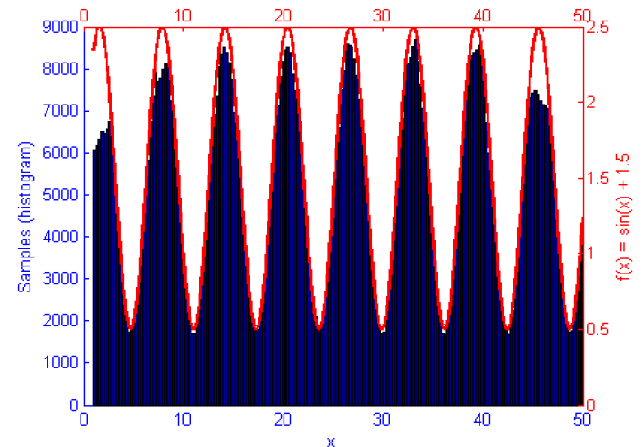
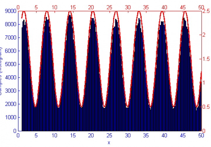
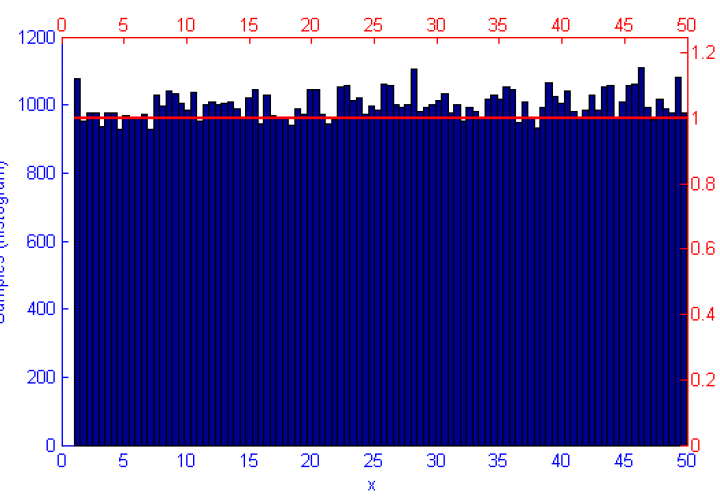
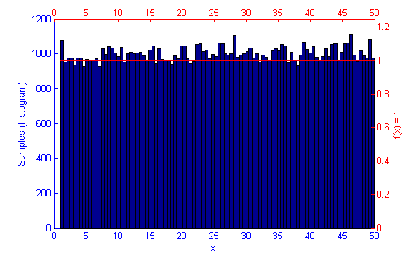
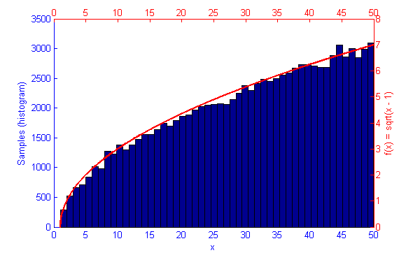
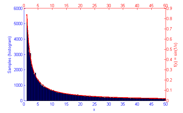
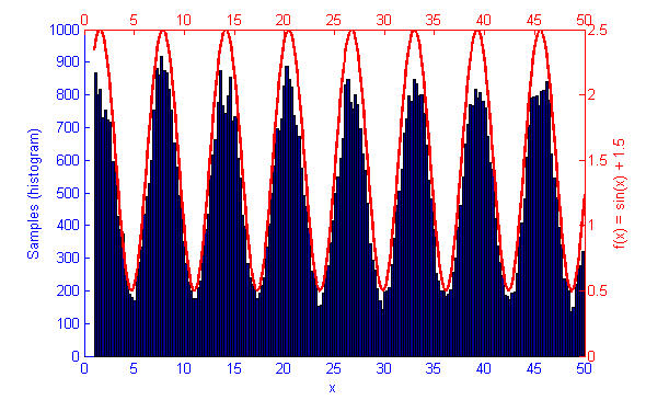
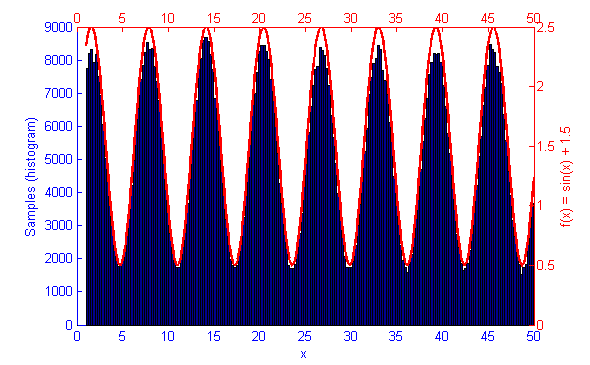
The function f(x) is shown in green, the sample distribution in blue with histogram bins marked as circles, and the error curve in orange. Since creating these images I’ve begun drawing the error on the log x log scale which displays as a linear decay as you’d expect.
Continuing on from experiments last week with Metropolis Hastings sampling for probability distributions I decided to implement Accept-Reject sampling. Accept-Reject seems to deliver well distributed results faster than Metropolis Hastings does but in the long run can easily introduce biased samples if the proposal distribution q(x) is not well tuned to the specific probability distribution function. MH on the other hand, is far more resilient to an improperly chosen proposal distribution as it will still converge to an unbiased result in most cases, albeit by taking a longer time to converge than it normally would. Accept-Reject also seems to have issues towards the truncations of it’s function causing under-sampling of values close to the lower and upper bounds.
A little update on what I’ve been learning about lately.
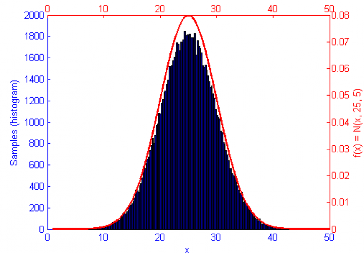
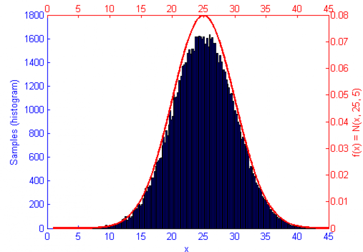
Metropolis-Hastings is an algorithm for sampling random values out of a probability distribution. Effectively, for a function f(x) you wish to simulate where the curve is higher it is more probable that a random number will be chosen from there. Uniform sampling of the range would mean that all x values on the graph have an even probability of being chosen, this could be simulated by saying f(x) = 1.
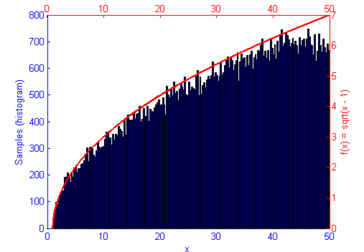
However, if the function f(x) represents a curve then the number of samples in high energy (probability) regions needs to be more dense. This can be seen in the simulations of f(x) = sqrt(x-1) and f(x) = sin(1/x) below.
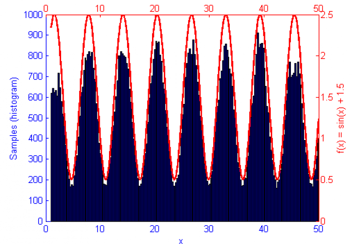
Metropolis-Hastings is best suited to problems where Direct Sampling and other more efficient solutions are not available. Because it only relies on the availability of a computable function f(x) and a proposal density Q(x|x*) M-H can correctly sample unusual probability distributions that would else-wise be difficult or impossible to compute. This can be seen below in the simulations of the sine function f(x) = sin(x) + 1.5.
Matlab code for Metropolis-Hastings Monte Carlo Integration (for generating samples)
Below is the Matlab code used to generate the above graph. By modifying the function f(x), the sample count N, the proposal distribution and it’s variance qV, and the upper and lower truncation bounds LB & HB any PDF can be simulated.