Yesterday I stumbled upon a lesser known and far superior method for mapping points from a square to a disk. The common approach which is presented to you after a quick google for Draw Random Samples on a Disk is the clean and simple mapping from Cartesian to Polar coordinates; i.e.
Given a disk centered origin (0,0) with radius r
// Draw two uniform random numbers in the range [0,1)
R1 = RAND(0,1);
R2 = RAND(0,1);

// Map these values to polar space (phi,radius)
phi = R1 * 2PI;
radius = R2 * r;

// Map (phi,radius) in polar space to (x,y) in Cartesian space
x = cos(phi) * radius;
y = sin(phi) * radius;
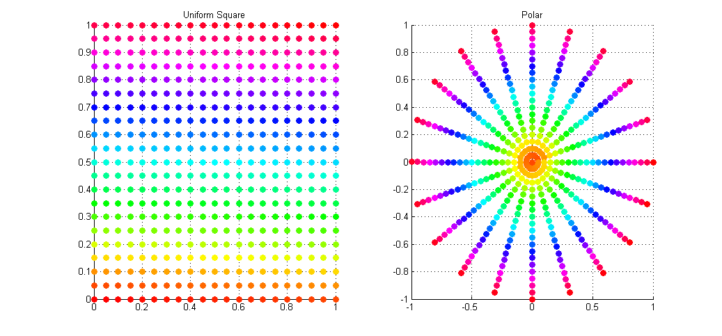
The result of this sampling on a regular grid of samples is shown in the image below. The left plot shows the input points as simple ordered pairs in the range [0,1)^2, while the right plot shows these same points (colour for colour) mapped onto a unit disk using Polar mapping as described above.
As you can see the mapping is not ideal with many points being over-sampled at the poles (I wonder why they call is Polar coordinates), and with areas towards the radius left under-sampled. What we would actually like is a disk sampling strategy that keeps the uniformity seen in the square distribution while mapping the points onto the disk.
Enter, Concentric Disk Sampling. This paper by Shirley & Chiu presents the idea for warping the unit square into that of a unit circle. Their method is nice but it contains a lot of nested branching for determining which quadrant the current point lays within. Shirley mentions an improved variant of this mapping on his blog, accredited to Dave Cline. Cline’s method only uses one if-else branch and is simpler to implement.
Again, given a disk centered origin (0,0) with radius r
// Draw two uniform random numbers in the range [0,1)
R1 = RAND(0,1);
R2 = RAND(0,1);

// Avoid a potential divide by zero
if (R1 == 0 && R2 == 0) {
    x = 0; y = 0;
    return;
}

// Initial mapping
phi = 0; radius = r;
a = (2 * R1) - 1;
b = (2 * R2) - 1;

// Uses squares instead of absolute values
if ((a*a) > (b*b)) {
    // Top half
    radius  *= a;
    phi = (pi/4) * (b/a);
}
else {
    // Bottom half
    radius *= b;
    phi = (pi/2) - ((pi/4) * (a/b));
}

// Map the distorted Polar coordinates (phi,radius)
// into the Cartesian (x,y) space
x = cos(phi) * radius;
y = sin(phi) * radius;
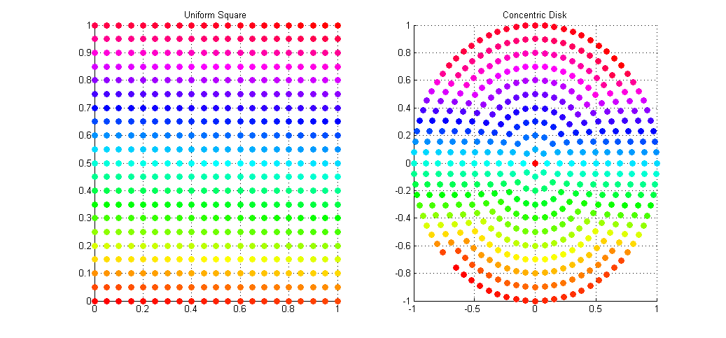
This gives a uniform distribution of samples over the disk in Cartesian space. The result of the mapping applied to the same set of uniform square samples is shown above. Notice how we now get full coverage of the disk using just as many samples, and that each point has (relatively) equal distance to all of it’s neighbors, meaning no bunching at the poles, and no under-sampling at the fringe.
I’ve applied this sampling technique to my Path Tracer as a means of sampling the aperture of the virtual point camera when computing depth of field. Convergence to the true out-of-focus light distribution is now much faster and more accurate than it was with Polar sampling which, due to bunching at the poles, cause a disproportionate number of rays to be fired along trajectories very close to the true ray.
It’s been a couple of weeks since I stopped working directly on rendering and took some time to read up on a topic called Hamiltonian (Hybrid) Monte Carlo which is to be the main focus of my research for the foreseeable future.
Hamiltonian Monte Carlo comes from a physics term of the same genesis called Hamiltonian Dynamics. The general idea being that, like with a Lagrangian equation for a system, you find a way to model the energy of a system which allows you to estimate it at efficiently even when the system is highly dimensional. With a Lagrangian you aim to minimize the degrees of freedom to reduce computation, and similarly with a Hamiltonian you reduce the problem to a measure of the systems kinetic K(p) and potential U(x) energy. This allows you to describe the entire state of an arbitrarily dimensional system as the sum of these measures, i.e. H(x,p) = U(x) + K(p)
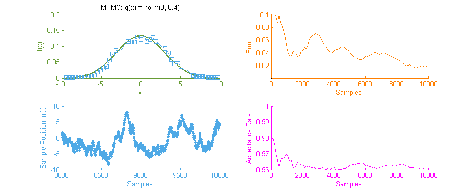
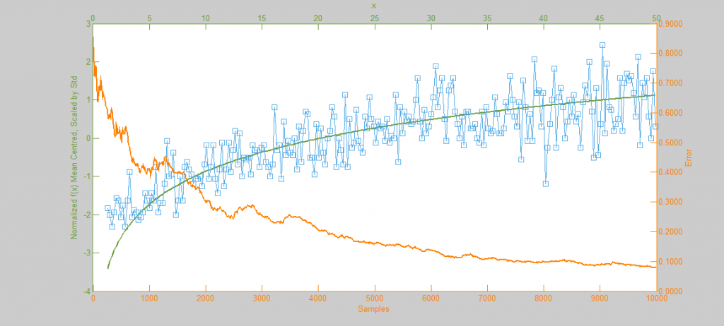
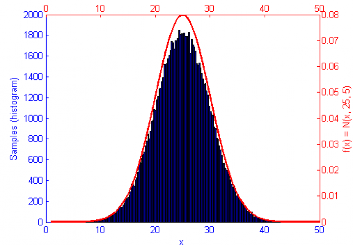
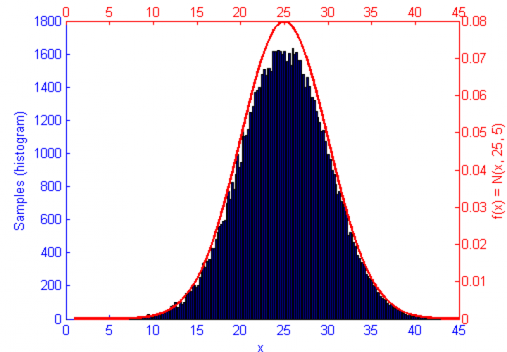
Above is our faithful companion, Metropolis Hastings Monte Carlo (MHMC), simulating a Normal distribution with mean “ and variance 3. The simulation was run for 10,000 samples yielding the shown results. Some things worth noting here are features such as the Error curve (Orange), which varies dramatically as simulation progresses. This is in-part due to the nature of the Random Walk which MHMC takes through the integration space which can be seen in the Blue graph to the bottom left. It is clear from the Blue graph that two states x and x' in the Makrov Chain are tightly dependent on one another.
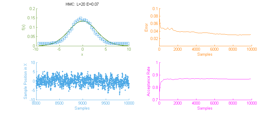
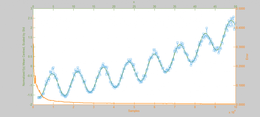
Next we see the same Normal distribution used above, estimated this time using Hamiltonian Monte Carlo (HMC) with trajectory length 20 and step size 0.07. To compare this to our previous simulation using MHMC several things become apparent. Firstly, The Error curve (Orange) seems to decay in a much more controlled and systematic manner. As opposed to the Error for MHMC which was erratic due to the nature of a Random Walk, here we see the benefit of making an informed choice as to where to place the next sample. From this we can hypothesise that a optimally tuned HMC simulation will in general reduce the error of the simulation with more samples consistently with little chance of introducing large, random, errors as with MHMC. Additionally in the sample placement graph (Blue) we see that the relationship between two states x and x' is far more abstracted, meaning two samples while being related and forming a valid Markov Chain will not reduce the accuracy of the simulation by treading on each others turf.
There is however, an issue with the above HMC simulation. Tuning. Unless properly tuned for the specific problem the Hyper-parameters for the Trajectory length L and Step size E will simply not work as intended and will yield poor results.
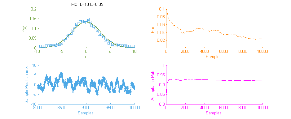
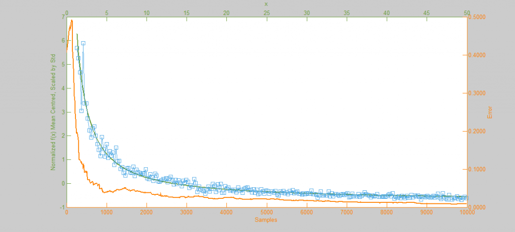
Above is a second run of the HMC simulation, this time with trajectory length 10 and step size 0.05. Because the length of the Leapfrog Trajectory was not sufficient to allow the system to move to an independent state we see the same banding of samples in the sample frequency graph (Blue) as we saw in the original Metropolis simulation. Additionally because of the dependent nature of the samples a similar pattern is seen in the Error curve (Orange) where the curve has large peaks where error was reintroduced to the system like with a Random Walk.
It is therefore vital to optimally tune HMC as the computation for each sample is an order of magnitude larger than with MHMC. Without proper tuning it’s much better to stick with the easier to tune MHMC.
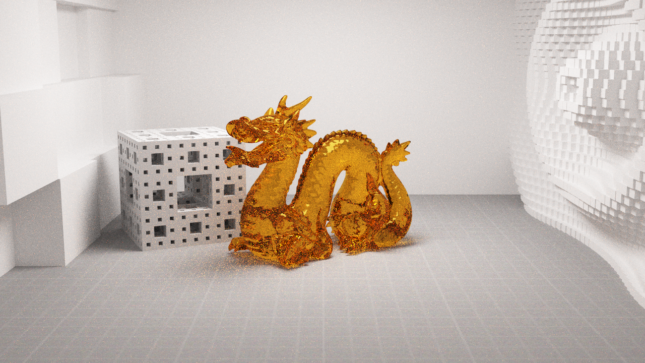
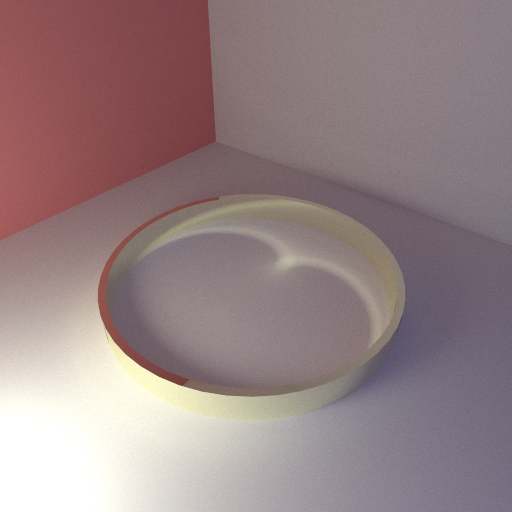
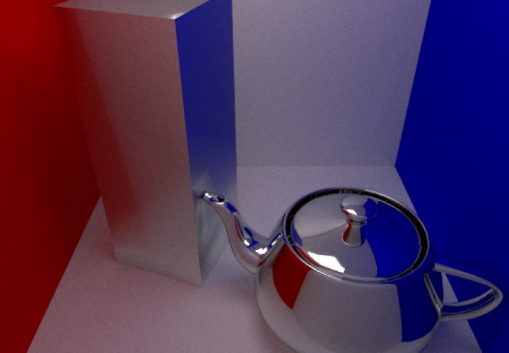
Thought it was about time to test some caustics on the renderer. Lately I’ve been both fascinated and frustrated by the strange forms and shapes that occur when light refracts and reflects off of lit surfaces. A great example of this is a metallic ring laying on a diffuse surface. Light bouncing onto the inside edge of the ring will be focused downwards onto the floor plane in a curved m shape causing a bright spot.
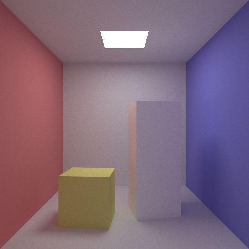
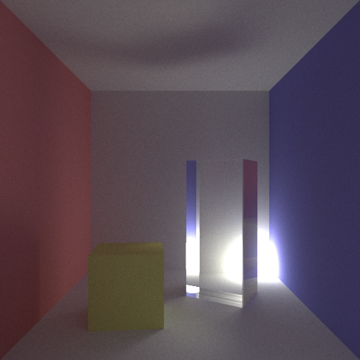
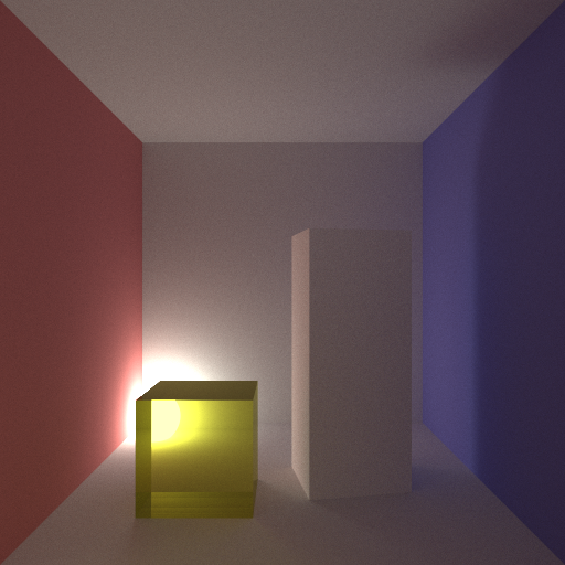
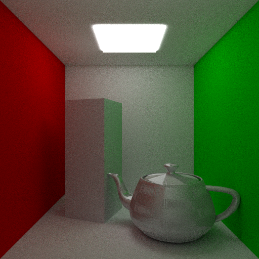
I’ve also been playing around with scenes that employ more indirect lighting. By this I mean scenes where the light source(s) are mostly if not entirely occluded from direct view by the camera. To this effect I set a standard cornell box scene with a yellow cube and a white oblong inspired by Cohen & Greenberg,and placed an occluded light sphere in the back-bottom corner of the room. I then toggled which of the two hemicubes were made of glass to see how the light would refract through them.
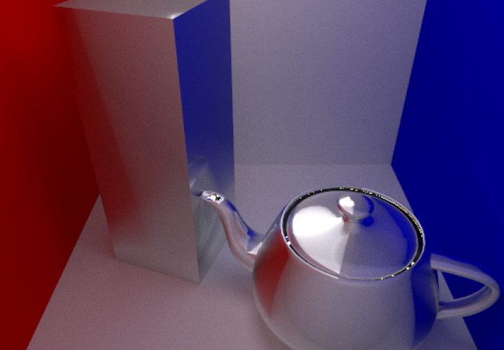
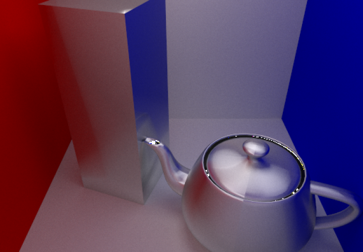
I thought I’d make some high quality comparison shots of some of the shaders I’ve been working on. Above you can see a side by side comparison of a perfect mirror BRDF and a Phong based BRDF with exponents of one million and ten for the centre and right images respectively.
While the Phong-like BRDF does give nice glossy reflections at a relatively small cost it does not model a physically accurate shader. I’m currently looking into implementing a Cook–Torrance model shader which while being more time consuming to compute gives nice results which are based off of physical phenomena. The Cook–Torrance shader also has the inherent ability to model microfacets within the surface of objects which is a big plus.
Because the Phong BRDF is not physically accurate I needed to find a PDF that would look correct in the renderings. The Mirror BRDF for instance has a PDF = 1 and the Diffuse BRDF has a PDF = 2 * (normal . newDirection). After some experimenting from reading a paper that claimed the Phong marginal pdf was cos(theta)^e which I understood (possibly incorrectly as it did not work) to mean PDF = (normal . newDirection)^e I found (gave up) that the Diffuse BRDF in fact worked reasonably well for the Phong model.
Edit I have found a better paper with what looks like a good Phong model. They even give a run down of using their model in a Monte Carlo style simulation with a marginal PDF. I might try implementing this before I move onto Cook-Torrance.
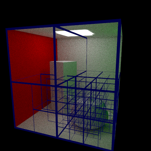
Previously I’ve debugged my KD-trees only by looking at archaic console printouts where at best each descending node in the structure is tabbed a couple of spaces further in from it’s parent.
However, seeing as I’m currently building a new renderer it seemed apt to build in a method for visualizing the generated trees. This was pretty simple to add in, if a preprocessor flag __AABB_EDGE__ is defined at compile time then during tree traversal additional code will run which does a simple UV coordinate calculation for the Axis Aligned-Bounding Box; if the UV is close enough to the edge of the box then the current pixel is abandoned and set to plain blue. The result is quite interesting to view and because of the power of the C++ preprocessor when it is disabled it effectively doesn’t exist in the compiled executable, meaning it has no effect on performance.
I have also been playing with specular and normal mapping. It was trivial to add due to the design of the shader class this time. In the case of specular mapping the max value of each RGB tuple is taken as the value for the map on the [0,1] range; this is then used to linearly scale the specular exponent of the shader which is used to calculate the glossy reflection for surfaces with an exponent > 0. Below a checker-board texture was used to scale a specular exponent of 128 into regions of 0 and 128 over the surface of the teapot.
So I’m still playing with graphs in Matlab… I shouldn’t complain, I know. I should be cherishing how laid back and relaxed the PhD experience is right now compared the where I’ll be a couple of years from now.
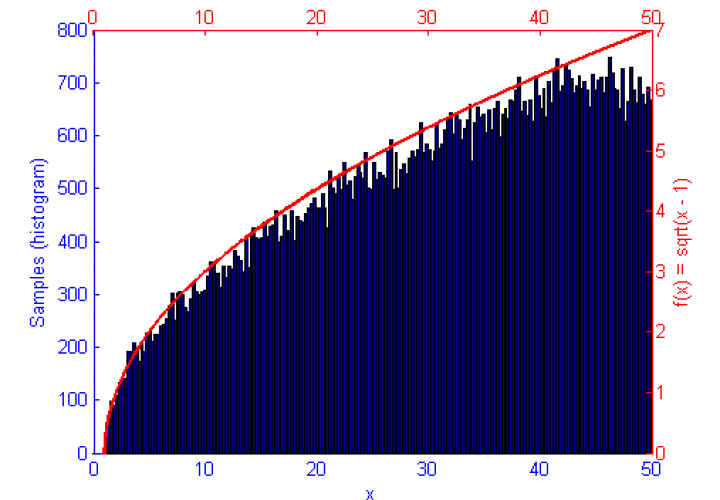
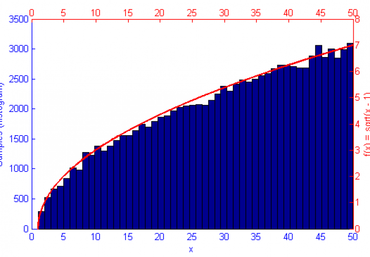
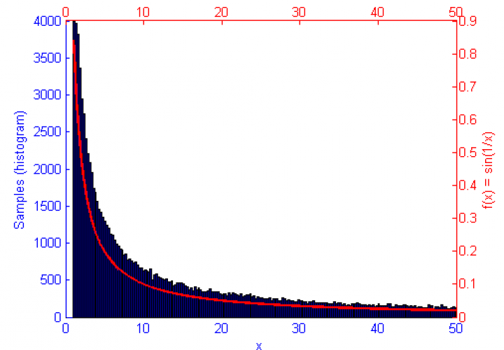
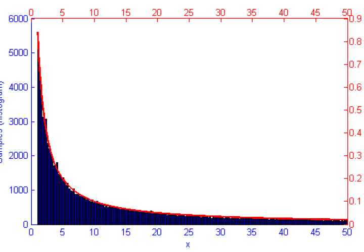
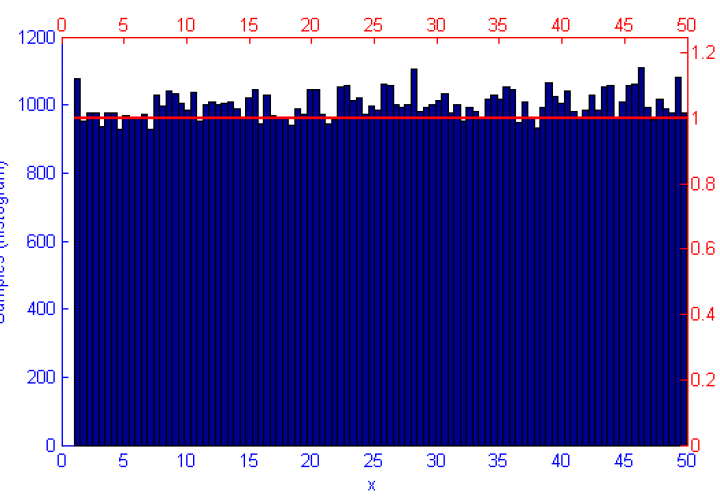
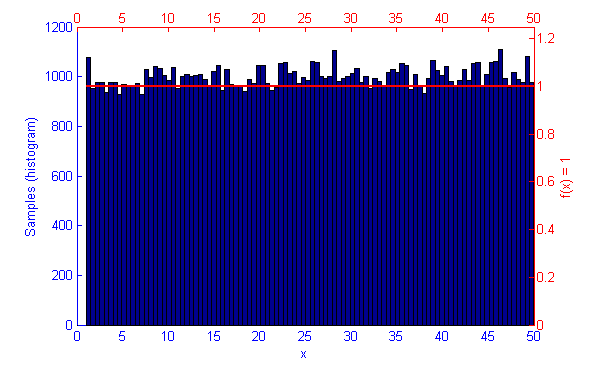
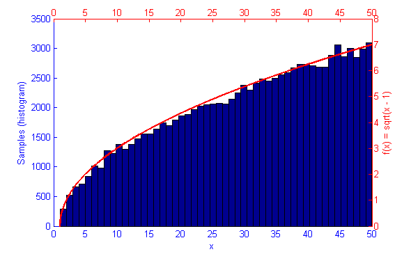
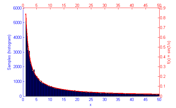
The function f(x) is shown in green, the sample distribution in blue with histogram bins marked as circles, and the error curve in orange. Since creating these images I’ve begun drawing the error on the log x log scale which displays as a linear decay as you’d expect.
Continuing on from experiments last week with Metropolis Hastings sampling for probability distributions I decided to implement Accept-Reject sampling. Accept-Reject seems to deliver well distributed results faster than Metropolis Hastings does but in the long run can easily introduce biased samples if the proposal distribution q(x) is not well tuned to the specific probability distribution function. MH on the other hand, is far more resilient to an improperly chosen proposal distribution as it will still converge to an unbiased result in most cases, albeit by taking a longer time to converge than it normally would. Accept-Reject also seems to have issues towards the truncations of it’s function causing under-sampling of values close to the lower and upper bounds.
A little update on what I’ve been learning about lately.
Metropolis-Hastings is an algorithm for sampling random values out of a probability distribution. Effectively, for a function f(x) you wish to simulate where the curve is higher it is more probable that a random number will be chosen from there. Uniform sampling of the range would mean that all x values on the graph have an even probability of being chosen, this could be simulated by saying f(x) = 1.
However, if the function f(x) represents a curve then the number of samples in high energy (probability) regions needs to be more dense. This can be seen in the simulations of f(x) = sqrt(x-1) and f(x) = sin(1/x) below.
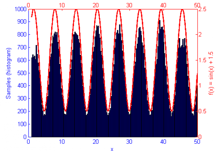
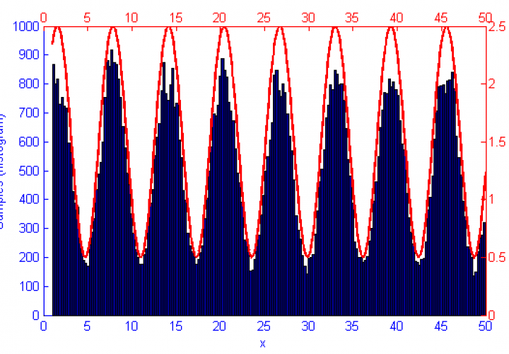
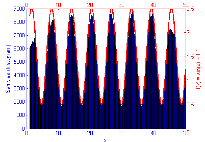
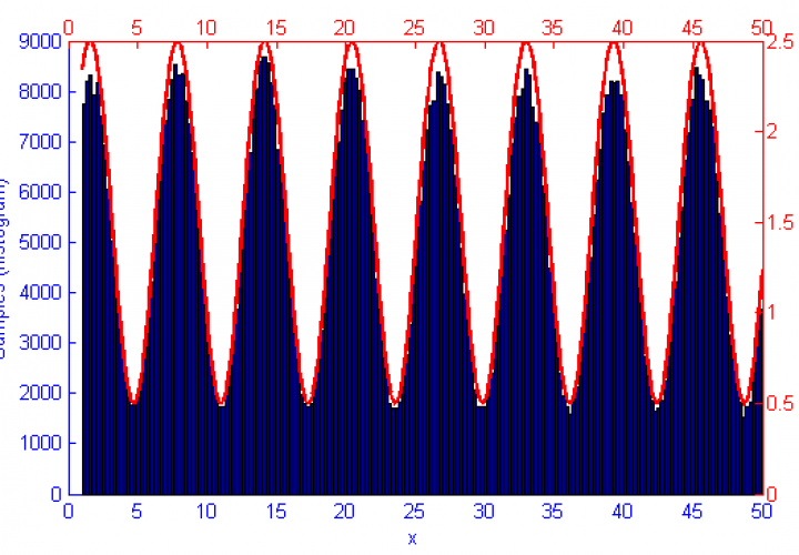
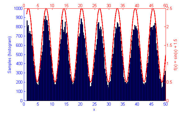
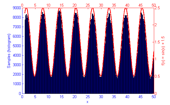
Metropolis-Hastings is best suited to problems where Direct Sampling and other more efficient solutions are not available. Because it only relies on the availability of a computable function f(x) and a proposal density Q(x|x*) M-H can correctly sample unusual probability distributions that would else-wise be difficult or impossible to compute. This can be seen below in the simulations of the sine function f(x) = sin(x) + 1.5.
Matlab code for Metropolis-Hastings Monte Carlo Integration (for generating samples)
Below is the Matlab code used to generate the above graph. By modifying the function f(x), the sample count N, the proposal distribution and it’s variance qV, and the upper and lower truncation bounds LB & HB any PDF can be simulated.