
Concentric Disk Sampling
December 22, 2014 - 10:49 am by Joss Whittle C/C++ Graphics Maths for Comp Sci Matlab PhD UniversityYesterday I stumbled upon a lesser known and far superior method for mapping points from a square to a disk. The common approach which is presented to you after a quick google for Draw Random Samples on a Disk is the clean and simple mapping from Cartesian to Polar coordinates; i.e.
Given a disk centered origin (0,0) with radius r
// Draw two uniform random numbers in the range [0,1)
R1 = RAND(0,1);
R2 = RAND(0,1);

// Map these values to polar space (phi,radius)
phi = R1 * 2PI;
radius = R2 * r;

// Map (phi,radius) in polar space to (x,y) in Cartesian space
x = cos(phi) * radius;
y = sin(phi) * radius;
The result of this sampling on a regular grid of samples is shown in the image below. The left plot shows the input points as simple ordered pairs in the range [0,1)^2, while the right plot shows these same points (colour for colour) mapped onto a unit disk using Polar mapping as described above.
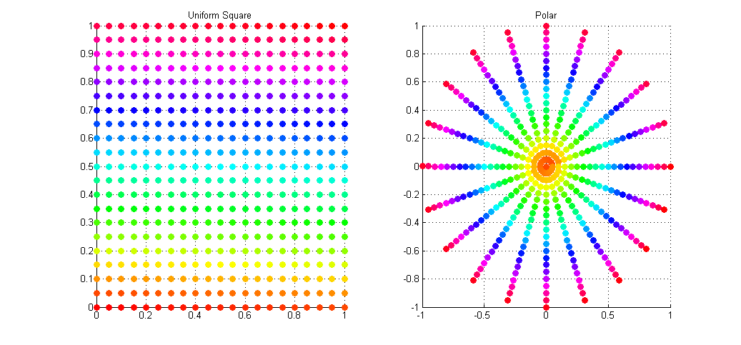
As you can see the mapping is not ideal with many points being over-sampled at the poles (I wonder why they call is Polar coordinates), and with areas towards the radius left under-sampled. What we would actually like is a disk sampling strategy that keeps the uniformity seen in the square distribution while mapping the points onto the disk.
Enter, Concentric Disk Sampling. This paper by Shirley & Chiu presents the idea for warping the unit square into that of a unit circle. Their method is nice but it contains a lot of nested branching for determining which quadrant the current point lays within. Shirley mentions an improved variant of this mapping on his blog, accredited to Dave Cline. Cline’s method only uses one if-else branch and is simpler to implement.
Again, given a disk centered origin (0,0) with radius r
// Draw two uniform random numbers in the range [0,1)
R1 = RAND(0,1);
R2 = RAND(0,1);

// Avoid a potential divide by zero
if (R1 == 0 && R2 == 0) {
    x = 0; y = 0;
    return;
}

// Initial mapping
phi = 0; radius = r;
a = (2 * R1) - 1;
b = (2 * R2) - 1;

// Uses squares instead of absolute values
if ((a*a) > (b*b)) {
    // Top half
    radius  *= a;
    phi = (pi/4) * (b/a);
}
else {
    // Bottom half
    radius *= b;
    phi = (pi/2) - ((pi/4) * (a/b));
}

// Map the distorted Polar coordinates (phi,radius)
// into the Cartesian (x,y) space
x = cos(phi) * radius;
y = sin(phi) * radius;
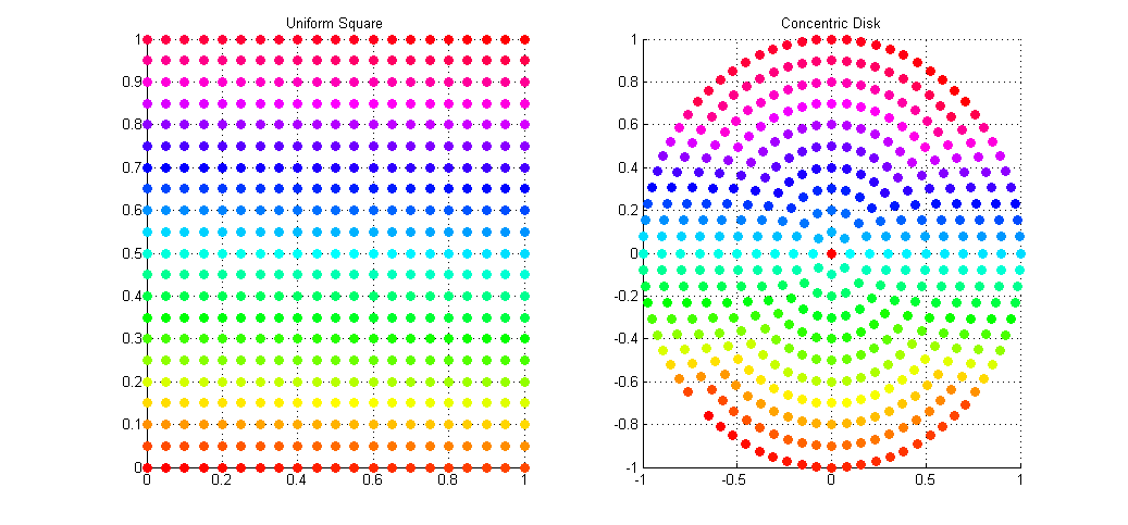
This gives a uniform distribution of samples over the disk in Cartesian space. The result of the mapping applied to the same set of uniform square samples is shown above. Notice how we now get full coverage of the disk using just as many samples, and that each point has (relatively) equal distance to all of it’s neighbors, meaning no bunching at the poles, and no under-sampling at the fringe.
I’ve applied this sampling technique to my Path Tracer as a means of sampling the aperture of the virtual point camera when computing depth of field. Convergence to the true out-of-focus light distribution is now much faster and more accurate than it was with Polar sampling which, due to bunching at the poles, cause a disproportionate number of rays to be fired along trajectories very close to the true ray.