Bunny Vase with Liquid
May 2, 2016 - 11:10 am by Joss Whittle C/C++ Graphics PhD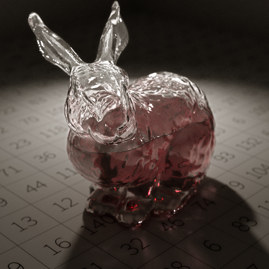

While working on my submission to this years SURF Research as Art Competition I realized that if I was to have any hope of rendering the final image at high resolution in a reasonable amount of time I would need more power. To do this I applied node parallelism in the form of a computer lab turned render farm.
The above image is the result of ~8 hours of rendering, at 4k resolution, over 18 machines (as described below). No colour correction or other post-processing (other than converting to jpeg for uploading) has been applied.
I try to keep the current generation of my rendering software nicely optimized but at it’s core it’s purpose is to be mathematically correct, capable of capturing a suite of internal statistics, and to be simple to extend. Speedup by cpu parallelism is only performed at the pixel (technically pixel tile) sampling level to reduce the amount of intrusion ray-packet tracing can bring to a renderer. In the future I plan to add a GPU work distributor using CUDA but for now this is quite low on my research priorities.
In order to get the speed boost I needed to render high resolution bi-directional path traced images I made use of Swansea Computer Sciences – Linux Lab, which has 30 or so i7, 8GB Ram, 256GB SSD machines running OpenSUSE. I wrote a bash script which for each ip address in a machine_file (containing all ip’s in the farm) ssh’s into each system and starts the renderer as a background process, and another to ssh into all machines and stop the current render.
The render job on each node outputs to a unique binary partials file every 10 samples per pixel (at 4k resolution) to a common network directory, overwriting the files previous values. This file contains three int’s containing width, height, and samples respectively; followed by (width * height * 3) double precision numbers representing the row-column pixel data stored in BGR format.
The data in the file represents the average luminance of each pixel in HDR. A second utility program can be run at a later time to process all compatible partials files in the same directory and turn them into a single image. Which is then properly tone mapped, gamma corrected, and saved as a .bmp file. To combine two partials, the utility program simply performs the following equation for each pixel:
P_1,2 = ((P_1 * S_1) + (P_2 * S_2)) / (S_1 + S_2)
By repeating this process one by one (each partial file can be > 500MB) all partials in a directory can be aggregated together into a single consistent and unbiased image.
After succumbing to a bit of a slump in research productivity over the last week or two it feels great to be making progress again.
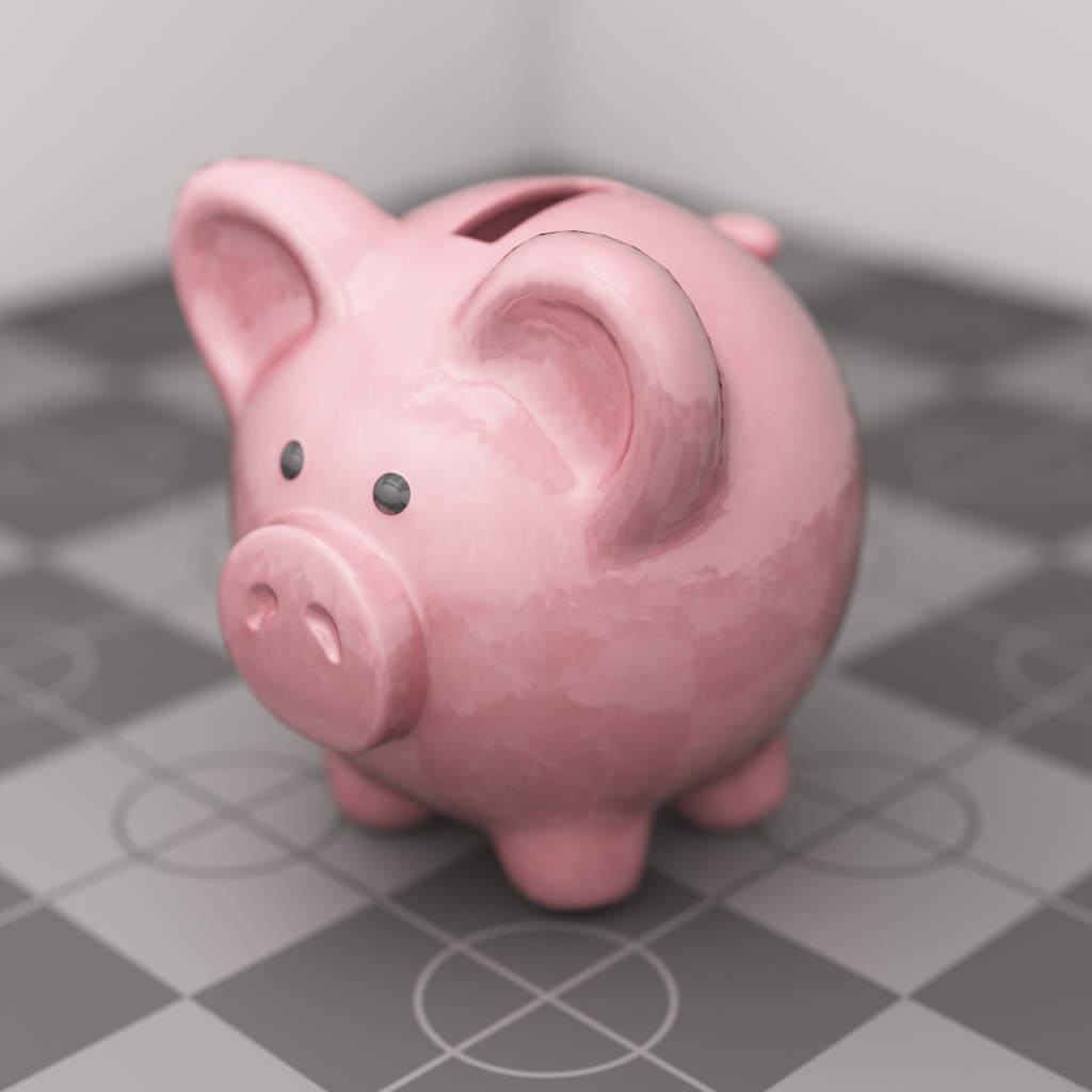
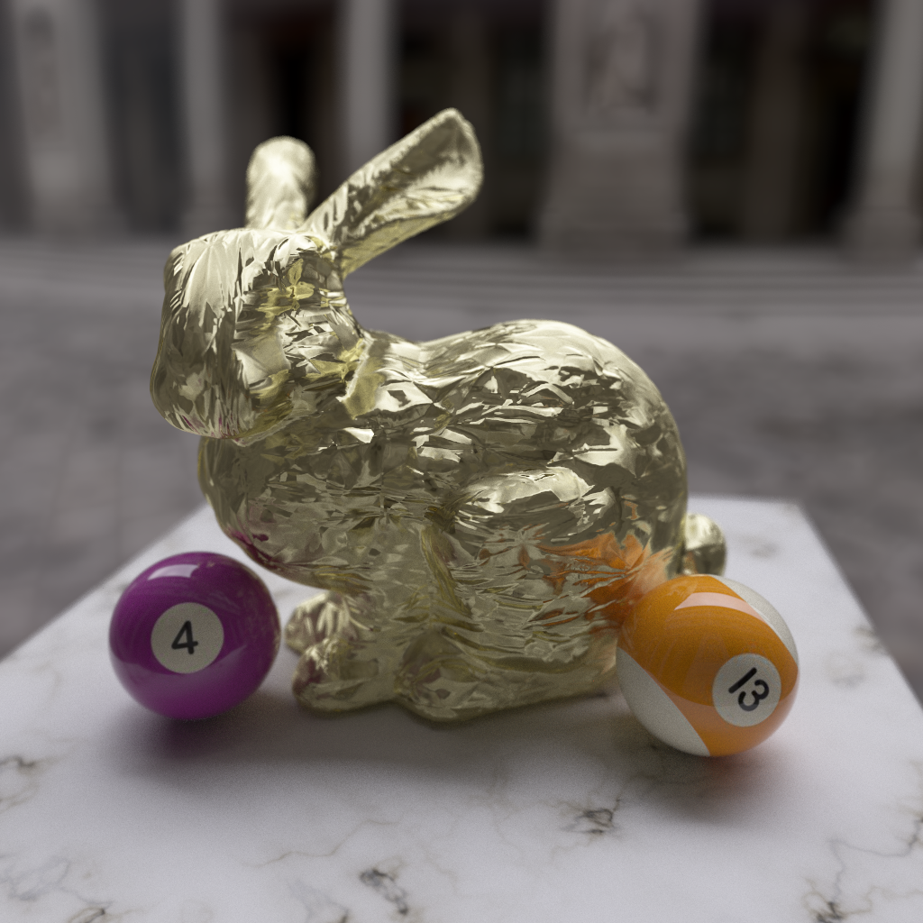
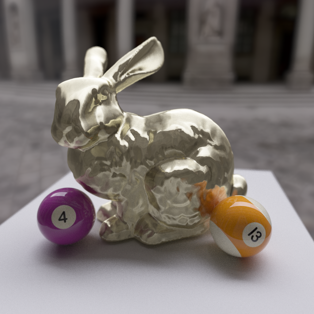
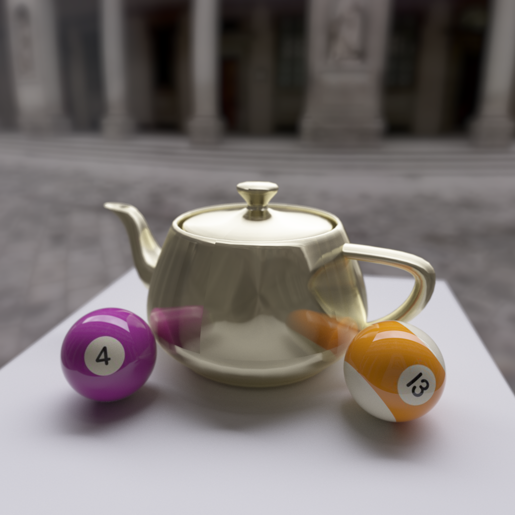
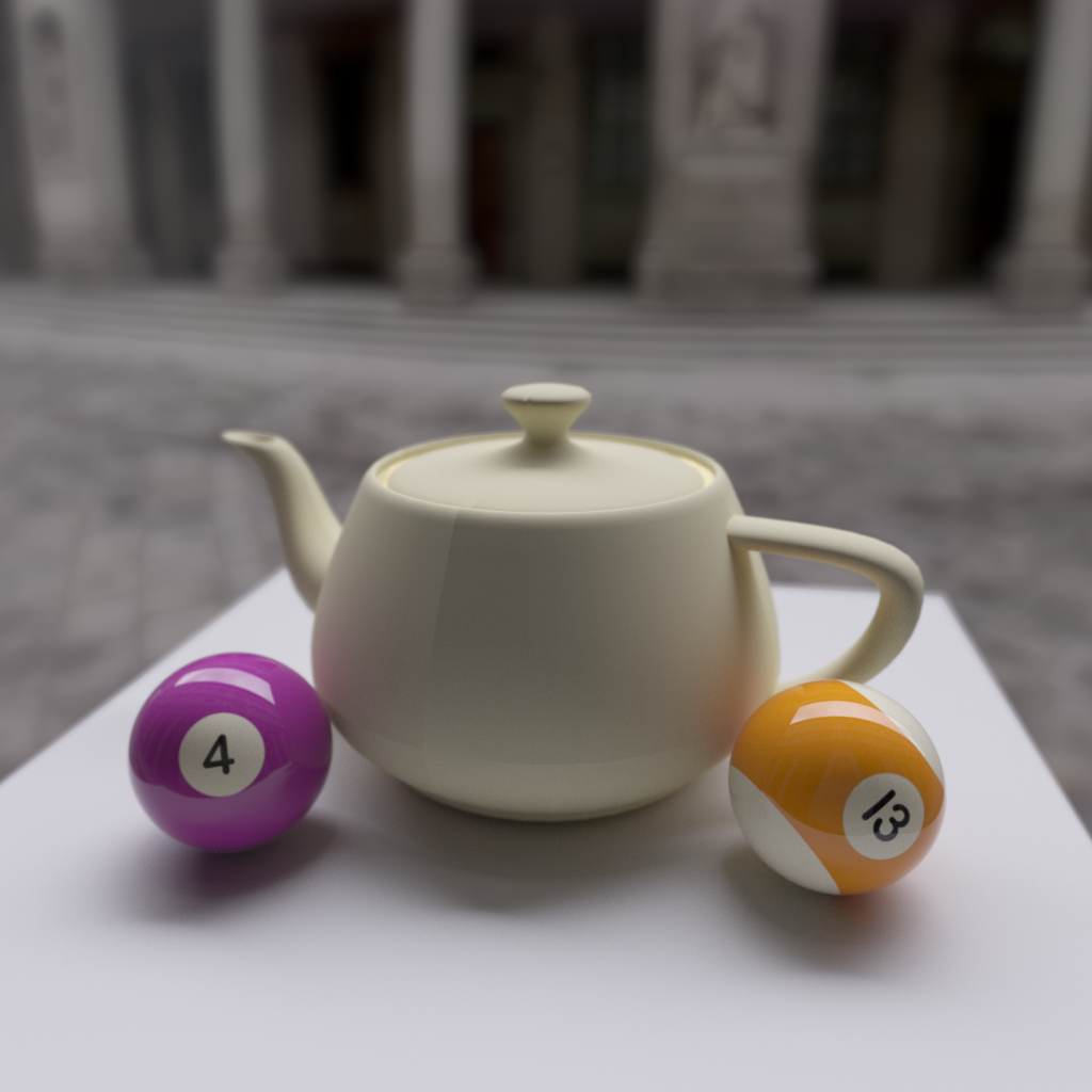
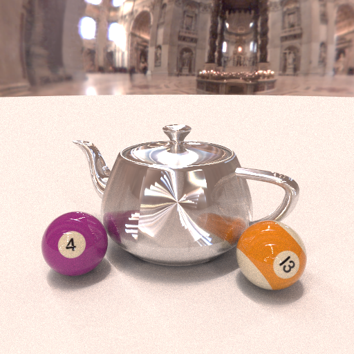
Finally I have a fully functional implementation of Bidirectional path tracing with some basic multiple importance sampling for the path weights. To celebrate having this new renderer in the code base I decided to have another crack at implementing a ceramic like shader. In the past I had modeled this material in geometry by placing a diffuse textured sphere inside an ever so slightly larger glass sphere to model the glaze/polish of the material. However, this method was a clunky approximation and severely limited the complexity of the models which it could be applied to.
This time I modeled a blended BRDF between a lambertian diffuse under-layer and an anisotropic glossy over-layer to represent the painted ceramic glaze. The amount of each BRDF used for each interaction is modulated by a Fresnel term on the incident direction. This means that looking straight at the surface will show mostly the coloured under-layer, while looking at glancing angles will show mostly the glossy over-layer.
The final, most important, part of this shader however is the bump map applied to it. Originally I rendered this scene without bump mapping, and while the material seemed plausible it looked almost too perfect. To break up the edges of reflections and to allow the surface of the material to “grab” onto a bit more light the effect of the material becomes and order of magnitude more convincing.
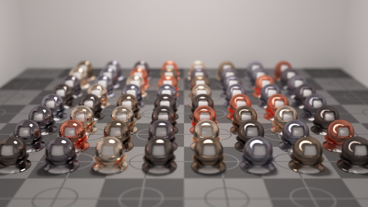
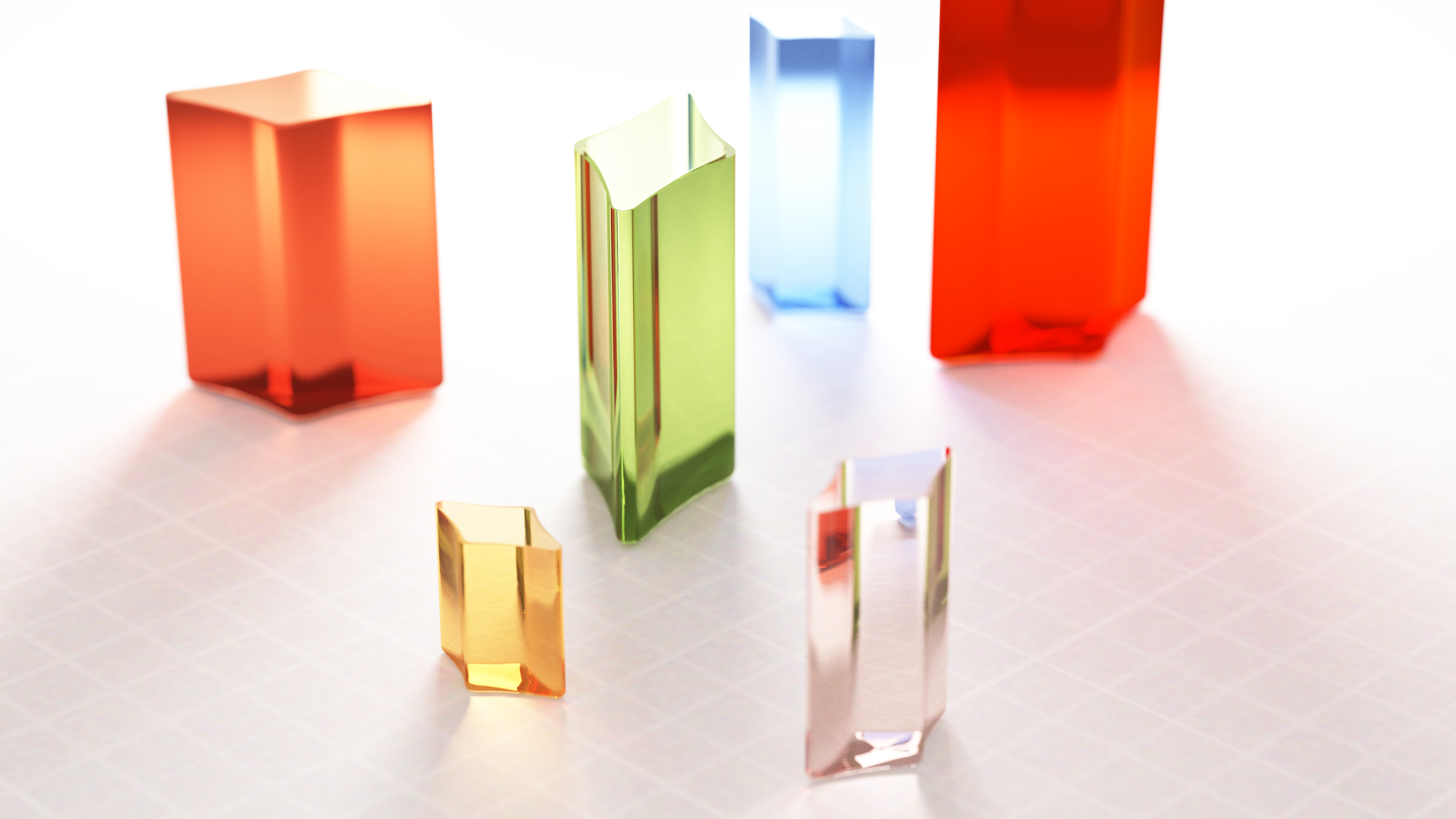
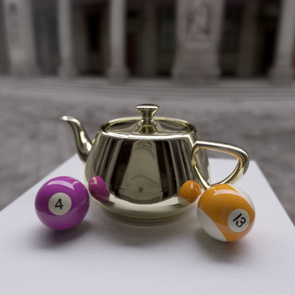
Just a quick render after implementing an Anisotropic Metal material in my renderer. The test scene was inspired by one I saw on Kevin Beason’s worklog blog.
Yesterday I stumbled upon a lesser known and far superior method for mapping points from a square to a disk. The common approach which is presented to you after a quick google for Draw Random Samples on a Disk is the clean and simple mapping from Cartesian to Polar coordinates; i.e.
Given a disk centered origin (0,0) with radius r
// Draw two uniform random numbers in the range [0,1)
R1 = RAND(0,1);
R2 = RAND(0,1);

// Map these values to polar space (phi,radius)
phi = R1 * 2PI;
radius = R2 * r;

// Map (phi,radius) in polar space to (x,y) in Cartesian space
x = cos(phi) * radius;
y = sin(phi) * radius;
The result of this sampling on a regular grid of samples is shown in the image below. The left plot shows the input points as simple ordered pairs in the range [0,1)^2, while the right plot shows these same points (colour for colour) mapped onto a unit disk using Polar mapping as described above.
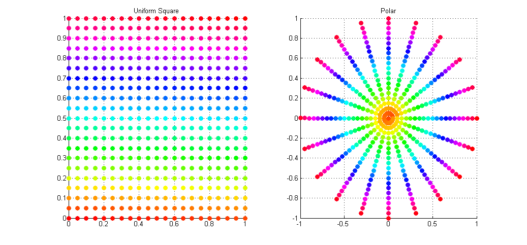
As you can see the mapping is not ideal with many points being over-sampled at the poles (I wonder why they call is Polar coordinates), and with areas towards the radius left under-sampled. What we would actually like is a disk sampling strategy that keeps the uniformity seen in the square distribution while mapping the points onto the disk.
Enter, Concentric Disk Sampling. This paper by Shirley & Chiu presents the idea for warping the unit square into that of a unit circle. Their method is nice but it contains a lot of nested branching for determining which quadrant the current point lays within. Shirley mentions an improved variant of this mapping on his blog, accredited to Dave Cline. Cline’s method only uses one if-else branch and is simpler to implement.
Again, given a disk centered origin (0,0) with radius r
// Draw two uniform random numbers in the range [0,1)
R1 = RAND(0,1);
R2 = RAND(0,1);

// Avoid a potential divide by zero
if (R1 == 0 && R2 == 0) {
    x = 0; y = 0;
    return;
}

// Initial mapping
phi = 0; radius = r;
a = (2 * R1) - 1;
b = (2 * R2) - 1;

// Uses squares instead of absolute values
if ((a*a) > (b*b)) {
    // Top half
    radius  *= a;
    phi = (pi/4) * (b/a);
}
else {
    // Bottom half
    radius *= b;
    phi = (pi/2) - ((pi/4) * (a/b));
}

// Map the distorted Polar coordinates (phi,radius)
// into the Cartesian (x,y) space
x = cos(phi) * radius;
y = sin(phi) * radius;
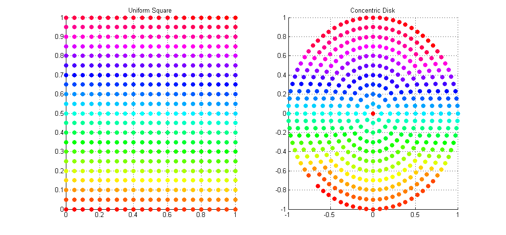
This gives a uniform distribution of samples over the disk in Cartesian space. The result of the mapping applied to the same set of uniform square samples is shown above. Notice how we now get full coverage of the disk using just as many samples, and that each point has (relatively) equal distance to all of it’s neighbors, meaning no bunching at the poles, and no under-sampling at the fringe.
I’ve applied this sampling technique to my Path Tracer as a means of sampling the aperture of the virtual point camera when computing depth of field. Convergence to the true out-of-focus light distribution is now much faster and more accurate than it was with Polar sampling which, due to bunching at the poles, cause a disproportionate number of rays to be fired along trajectories very close to the true ray.
Really pleased with the first functioning results from my Environment Sphere class. For variance reduction I’ve implemented a stippling method, drawing samples directly from the Inverse CDF of the image.
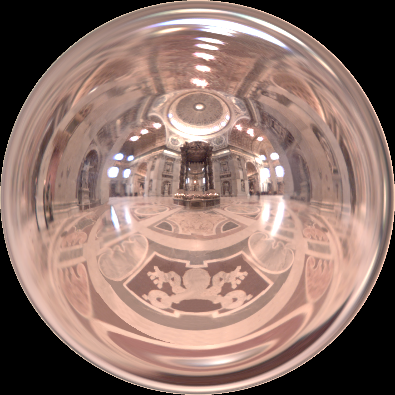
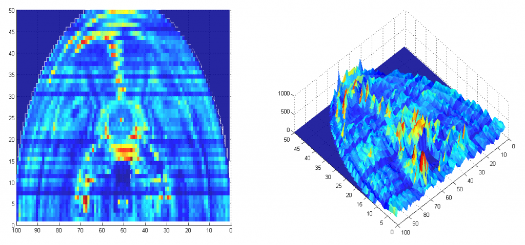
Or rather, I first generate a CDF of the Y axis where each value is the average brightness for the row. From this I invert to build an Inverse CDF for the axis. For each row in turn I generate the CDF and Inverse CDF and store them in a 2D matrix. To sample the image, you simple generate a uniform random number in the range v ~ Unif(0, Max avg row brightness in Y) and then lookup the corresponding value in the Inverse CDF of Y, y = icdfY[v]. This gives a randomly selected row in the image based on the probability the pixel with be bright, and thus contribute highly to the image. To complete the sampling we now find a random pixel at column x along row y by sampling the Inverse CDF of row y. We do this by drawing a second uniform random number u ~ Unif(0, Max Brightness of row Y) and use it to look up the corresponding pixel location in x, x = icdfX[y][u]. We now have a random pixel in the image drawn stochastically. Below is a visualization of how many samples were taken from each pixel area over the course of 1 million test samples. As you can see far more time is spent sampling pixels with high (bright) image contribution.
This can then easily be turned into a unit vector of the direction to the pixel when mapped onto a unit sphere. This is simply the XY coordinate mapped uniformly onto the range x,y = ((x / w, y / h) * 0.5) - 0.5 and then orthogonally projected onto the sphere along the Z axis; forming the vector V(x,y, abs(x) * (rand() < 0.5 ? -1 : 1) ) That is to say, we choose with a random probability whether the pixel is mapped to the near or far side of the sphere.
Potentially this could be optimized by then calculating the dot product between surface normal and the generated samples. If the face is culled we could immediately flip the vectors Z axis and potentially save the sample from being a waste of computation.