A more interesting Cornell Box
October 31, 2014 - 11:48 pm by Joss Whittle C/C++ Graphics PhD University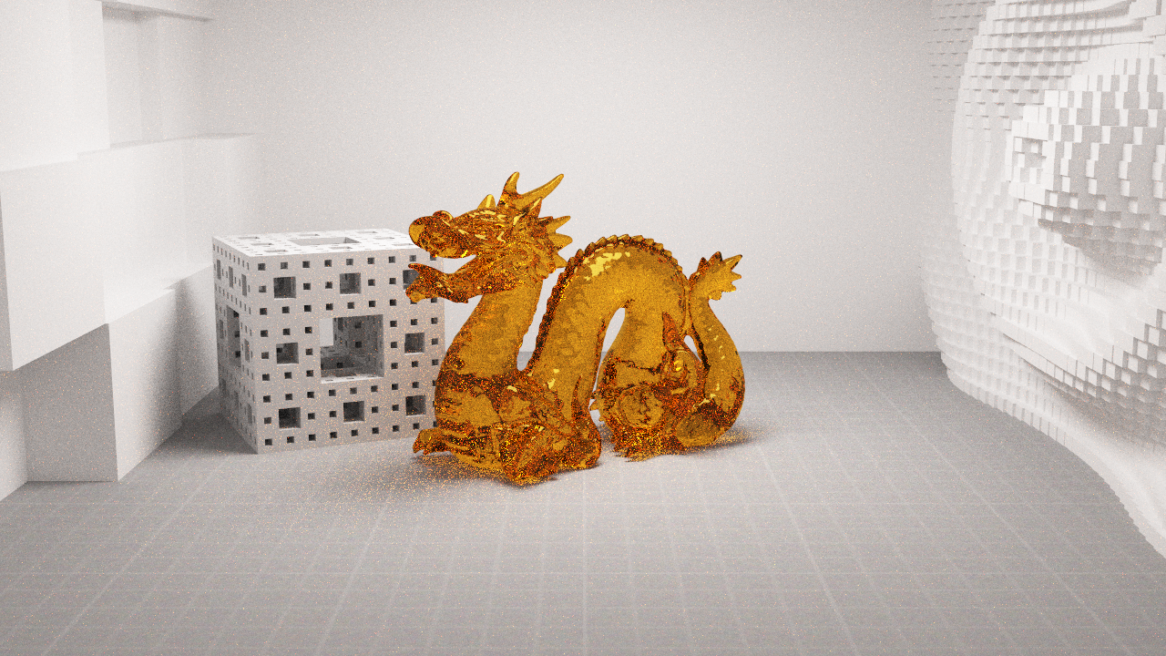

Really pleased with the first functioning results from my Environment Sphere class. For variance reduction I’ve implemented a stippling method, drawing samples directly from the Inverse CDF of the image.
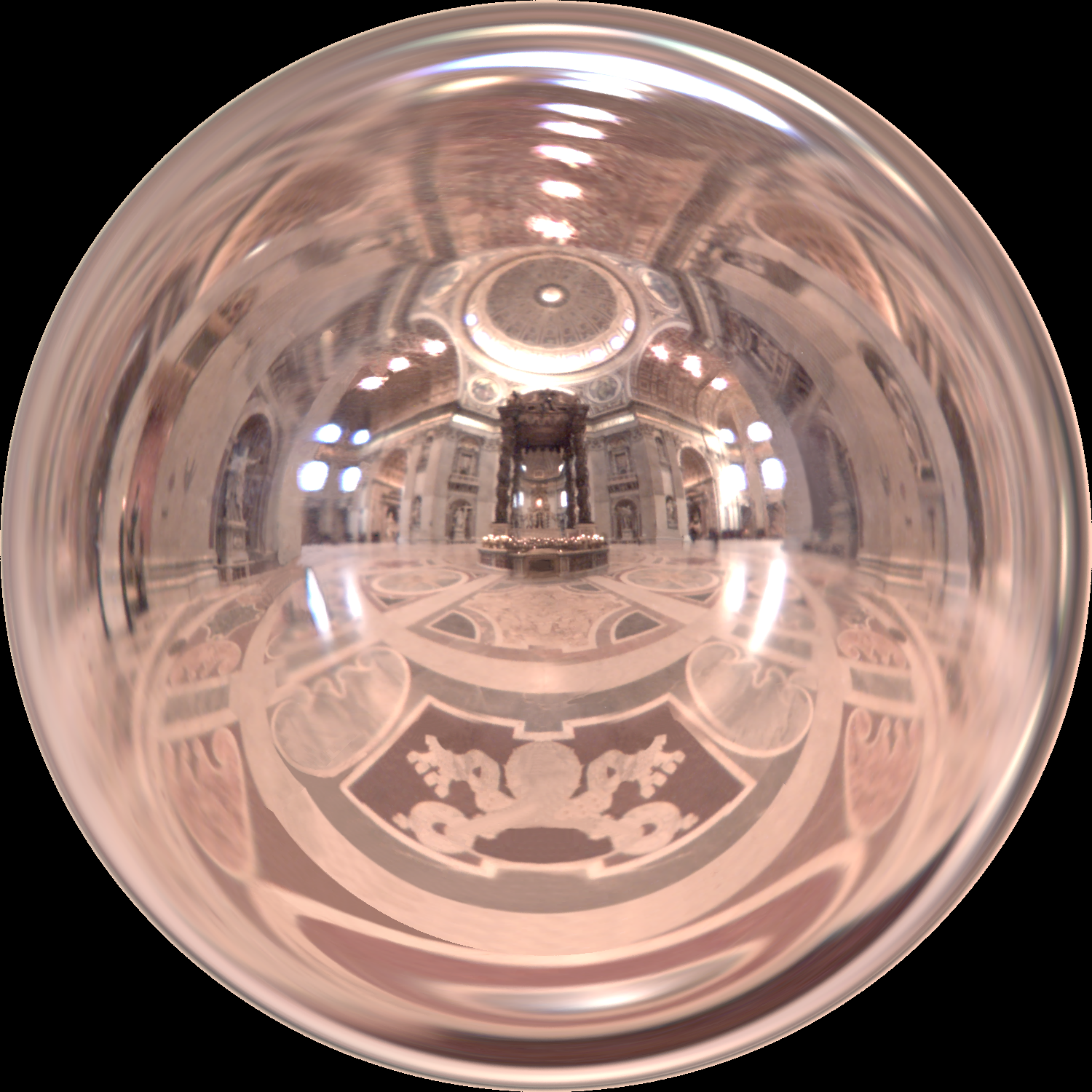
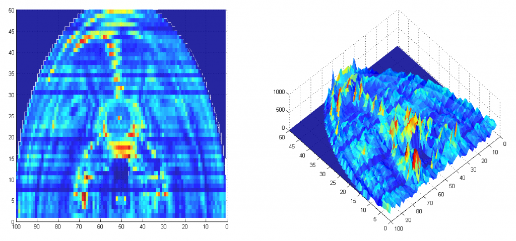
Or rather, I first generate a CDF of the Y axis where each value is the average brightness for the row. From this I invert to build an Inverse CDF for the axis. For each row in turn I generate the CDF and Inverse CDF and store them in a 2D matrix. To sample the image, you simple generate a uniform random number in the range v ~ Unif(0, Max avg row brightness in Y) and then lookup the corresponding value in the Inverse CDF of Y, y = icdfY[v]. This gives a randomly selected row in the image based on the probability the pixel with be bright, and thus contribute highly to the image. To complete the sampling we now find a random pixel at column x along row y by sampling the Inverse CDF of row y. We do this by drawing a second uniform random number u ~ Unif(0, Max Brightness of row Y) and use it to look up the corresponding pixel location in x, x = icdfX[y][u]. We now have a random pixel in the image drawn stochastically. Below is a visualization of how many samples were taken from each pixel area over the course of 1 million test samples. As you can see far more time is spent sampling pixels with high (bright) image contribution.
This can then easily be turned into a unit vector of the direction to the pixel when mapped onto a unit sphere. This is simply the XY coordinate mapped uniformly onto the range x,y = ((x / w, y / h) * 0.5) - 0.5 and then orthogonally projected onto the sphere along the Z axis; forming the vector V(x,y, abs(x) * (rand() < 0.5 ? -1 : 1) ) That is to say, we choose with a random probability whether the pixel is mapped to the near or far side of the sphere.
Potentially this could be optimized by then calculating the dot product between surface normal and the generated samples. If the face is culled we could immediately flip the vectors Z axis and potentially save the sample from being a waste of computation.
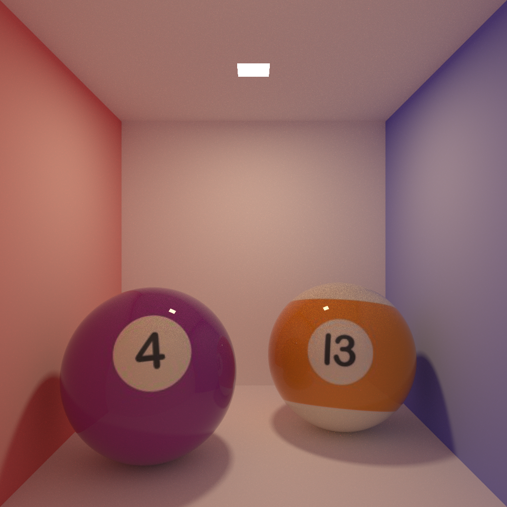
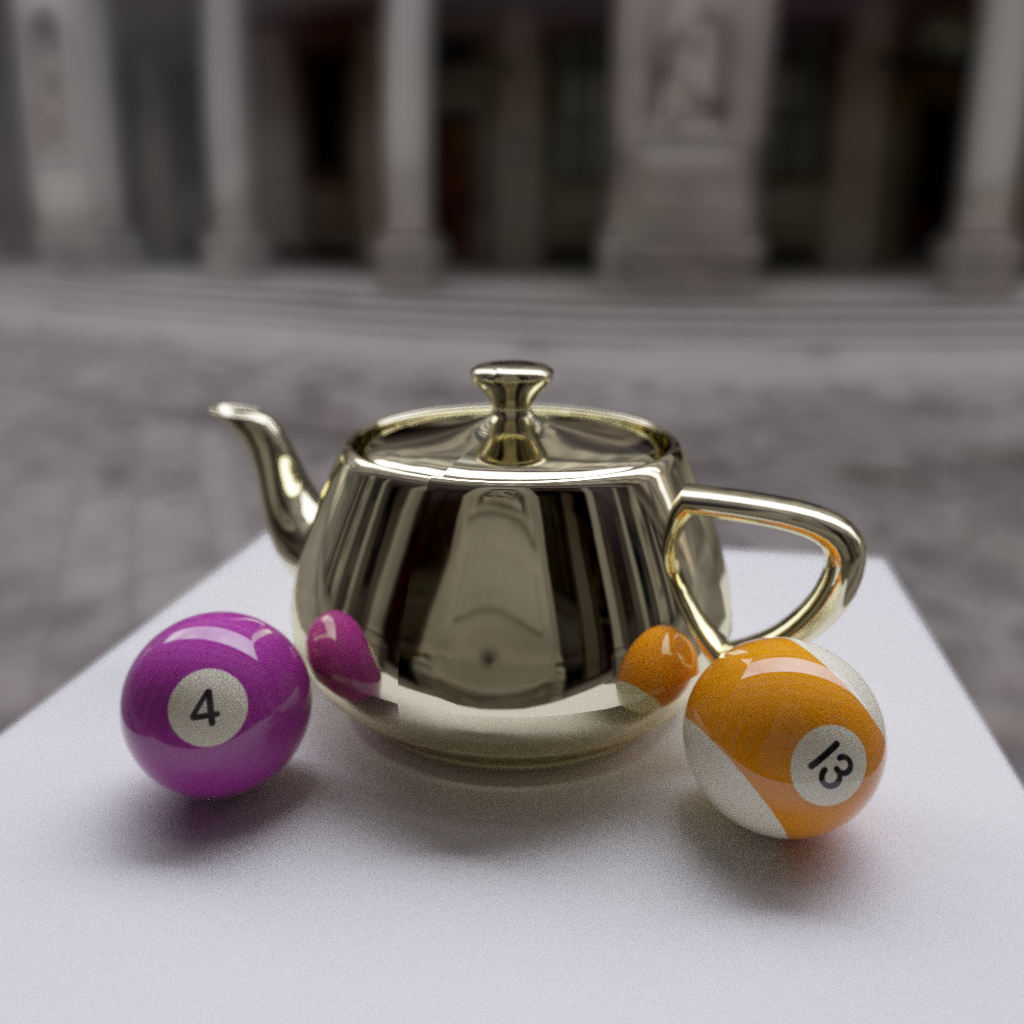
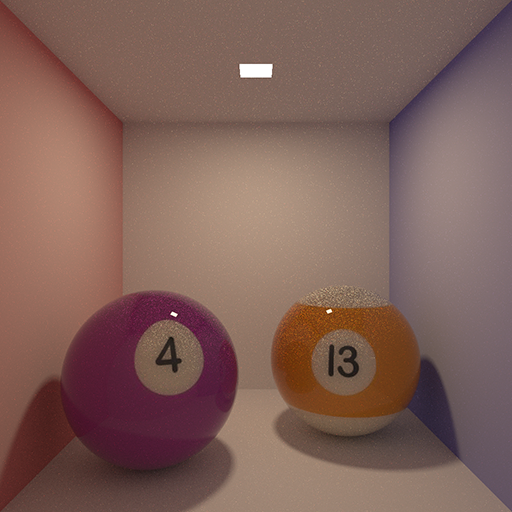
Here is a more converged render of the pool balls which I left running on my uni computer overnight. The image is 1024 x 1024 pixels and was rendered to 1250 samples over the course of around 4 hours.
There are also several notable changes that have been made to the renderer which show up in the new image. Firstly, the strange distortion of the texture on the sphere (visible on the ‘4’) has been fixed. This was due to an incorrect method of rotating the UV coordinates of the sphere around it’s centre. Previously this was accomplished by adding radians to the computed (phi, theta) coordinates. However, this was not a true rotation but rather a translation over the surface along the polar axis. So by attempting to lean the sphere backwards slightly I had really just shifted the texture slightly higher on the sphere.
The new method for rotating a sphere is defined below, it works by having a pair of ‘home’ vectors for the sphere. One pointing upwards towards the north pole, and the other point outwards at 90′ degrees towards the intersection of equator & the prime meridian.
The second change is the addition of Bi-Linear Interpolation on texture sampling. In my rush to get a minimum renderer working to begin research I skipped adding this and opted for the simple Nearest Neighbor approach by simply casting my computed texture coordinates to int‘s. However, as I am now beginning to produce higher quality renders it became painfully apparent how important a good texture lookup can be to final quality.
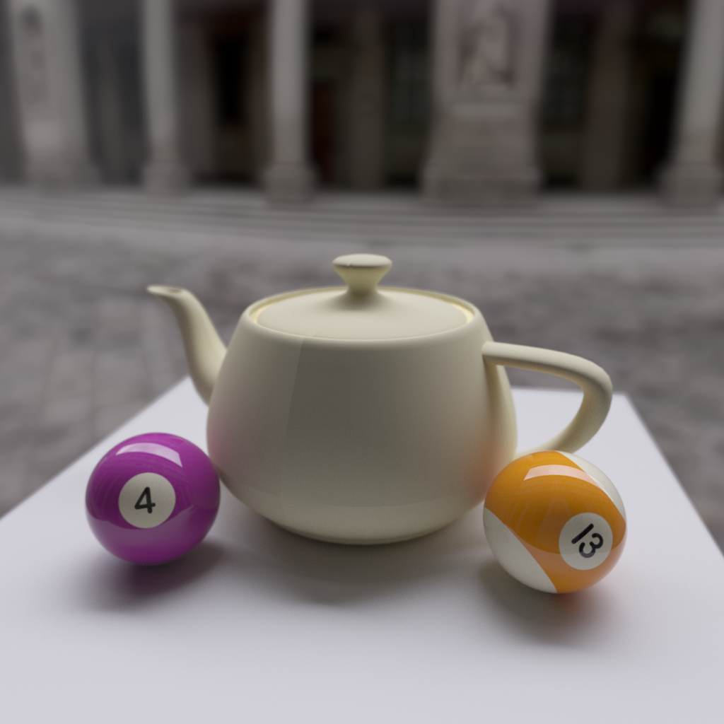
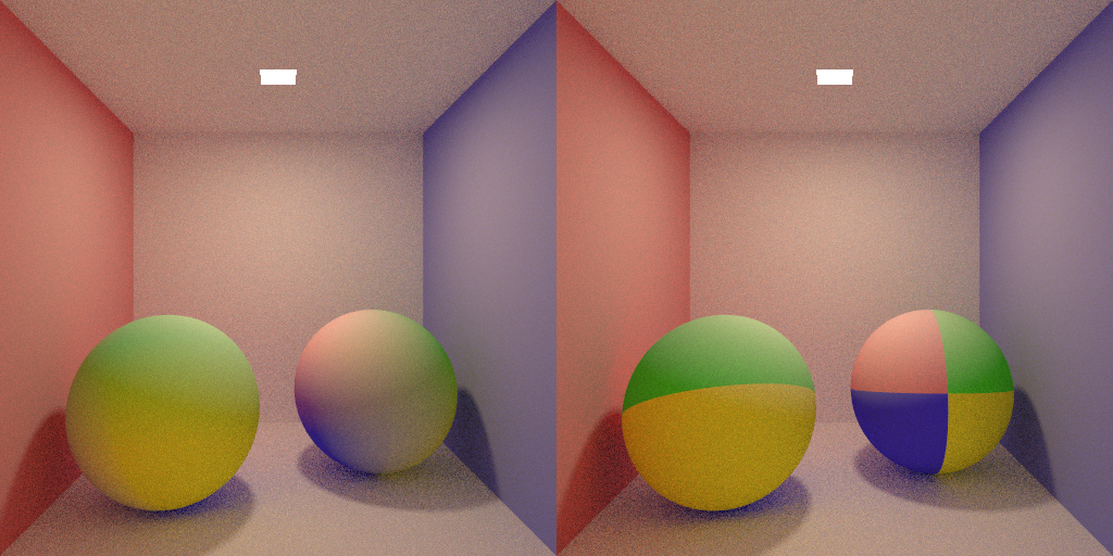
Below is a quick comparison of the previous image (left) and the new image (right). Other than the obvious texture distortion as mentioned above, you can also see how jagged the edges are where the texture changes colour dramatically. In the right hand image, however, the effect of Bi-Linear interpolations can be seen a subtle blurring as the colours change.
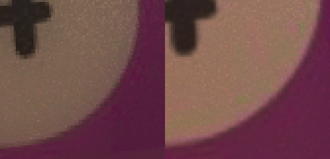
Here, an even more dramatic comparison is shown where a 2 x 2 pixel texture has been wrapped around the spheres. On the right, the colour of the sphere jumps dramatically between the four pixels of the texture while the left rendering shows a smooth transition between colours.
Here is the code for Bi-Linear Interpolation based on a set of UV texture coordinates in the range 0 -> 1.
Continuing on with my work implementing direct lighting contributions to the renderer I thought I’d take a second to show off some shots I’m most happy with.
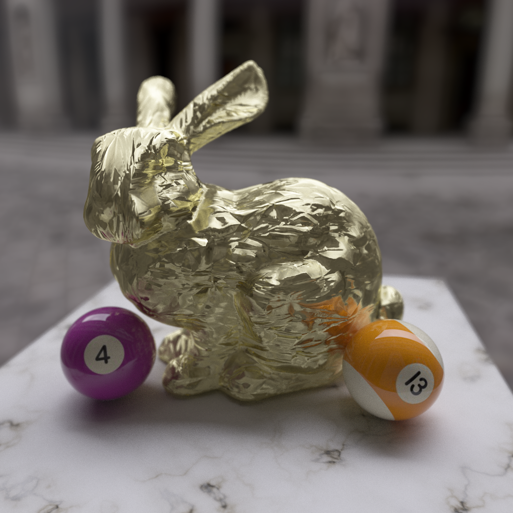
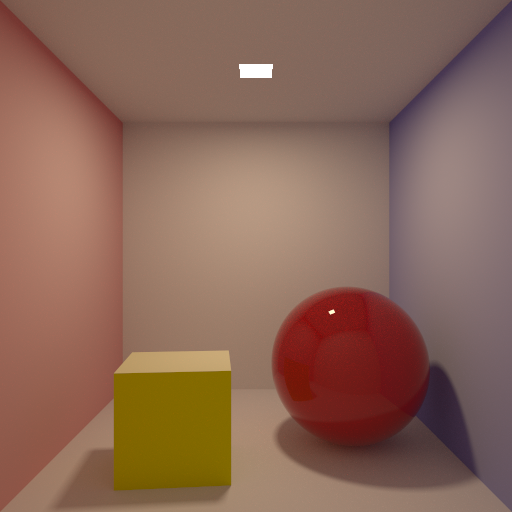
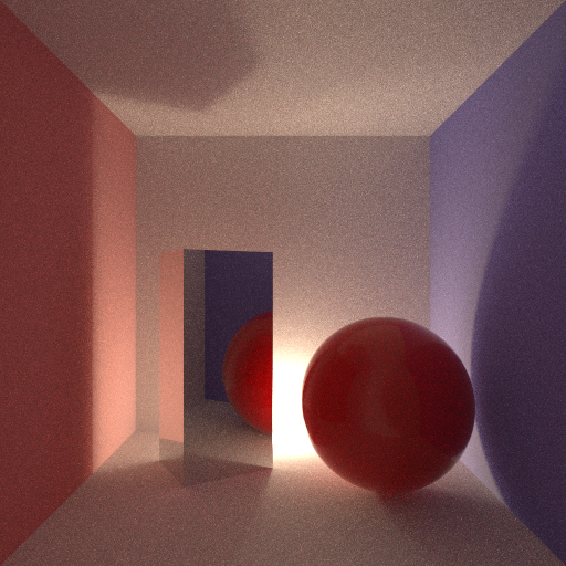
This first shot I am most pleased with, though it could possibly be subject bias due to my having stared at it for hours as I program; however, I am convinced this looks physically plausible. Or at least, it’s the most physically plausible thing I have rendered so far. This image was rendered using 1250 samples with a 1 unit thick coat of clear varnish on the diffuse red sphere.
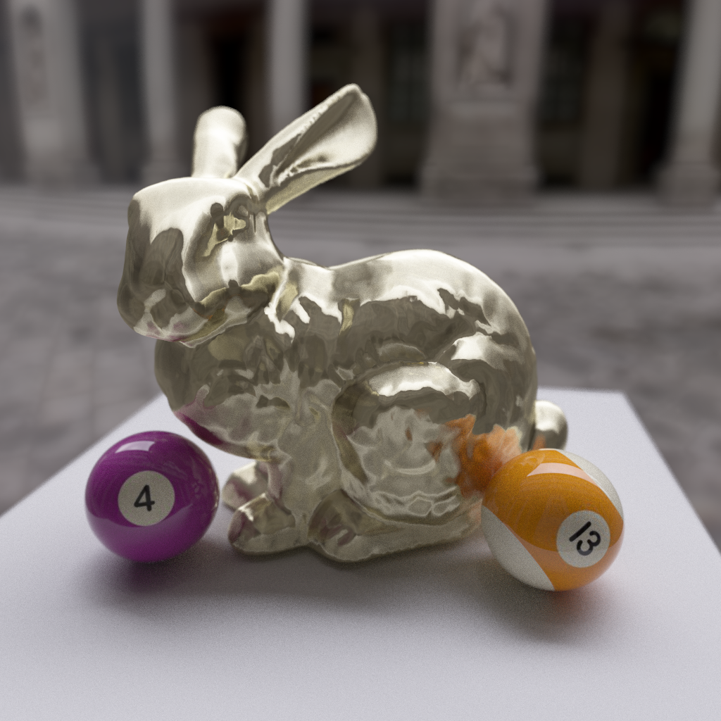
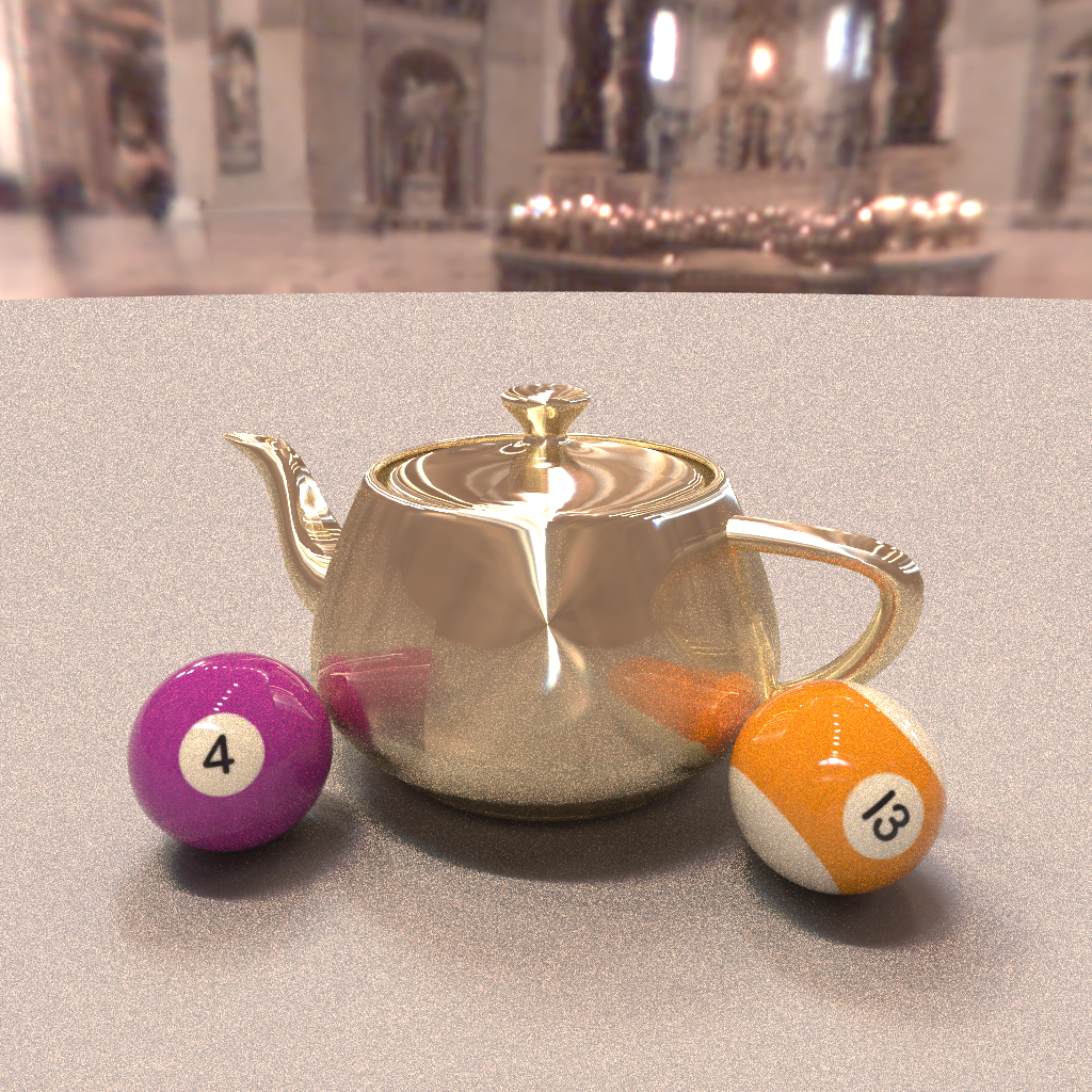
I decided to try combining the sphere shader with texture mapping to see how good it would look as a glossy stone shader. Due to the high variance from the two balls this image was rendered at 2x resolution (1024 x 1024) and then downsized back to the normal resolution. The upscaled image was rendered with 100 samples.
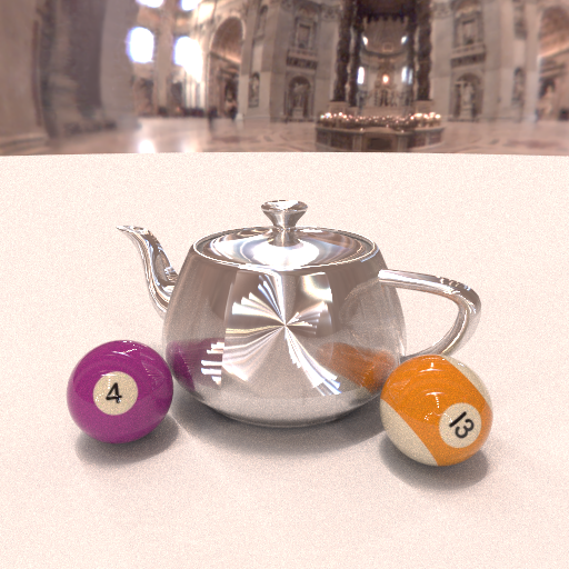
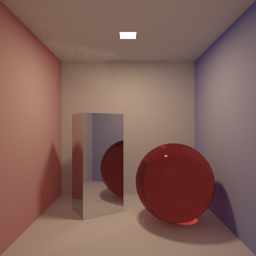
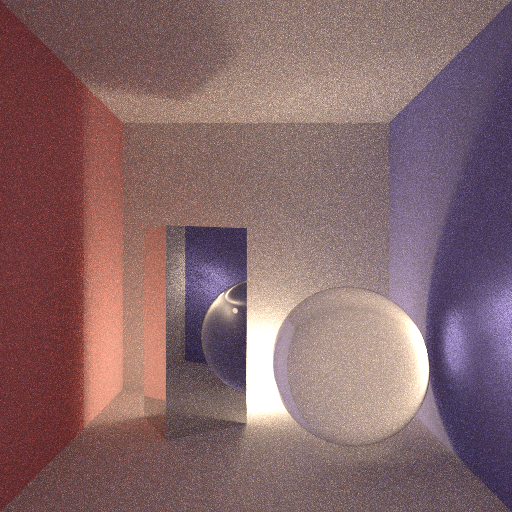
The next image was rendered using 1000 samples. Despite the increased convergence speed of the red glass sphere compared to the ceramic one in the first image, the presence of mirror box adds variance back into the image due to it’s broad specular caustics.
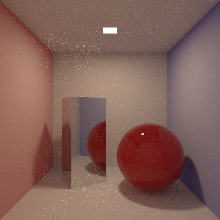
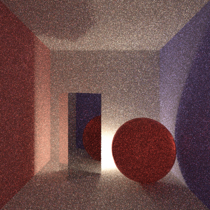
I also experimented with testing different light positions to see how robust the direct lighting contribution was compared to Naive Path Tracing alone. A more complete comparison of light positions using 25 samples per image is shown further down this post. For the next image, the light is placed on the floor along the rear wall of the Cornell Box. The shot was rendered with 1000 samples and 1 unit varnish on the sphere.
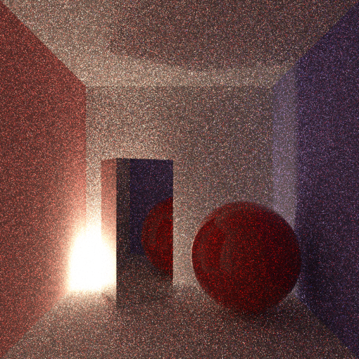
Next the same shot is shown, this time rendered with only 250 samples and a clear glass sphere. Even after this relatively small number of samples, well defined caustics can be seen on the right wall and on the surface of the sphere, indirectly, through the mirror box.
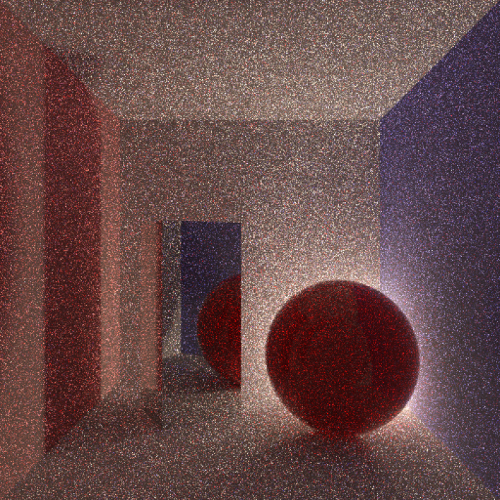
Below, four renders are shown with varying light positions. The overhead light is a 1 x 1 unit square which emits light uniformly in a downward facing hemisphere, while the three backlit images are lit by unit spheres placed just above the ground.
As you can see, while convergence is still impressive for such a low sample count using a small surface area light source, variance still remains a major issue. Now that I know the direct lighting calculation works however, I think it can be implemented into the Bi-Directional Path Tracer which should help solve some of it’s shading issues.
Finally starting to make up for the time I took off over christmas!
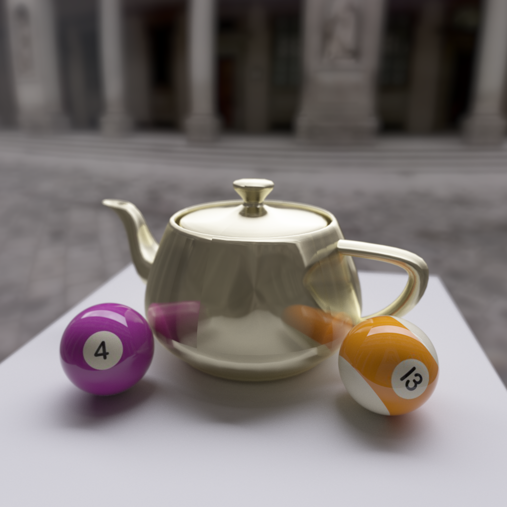
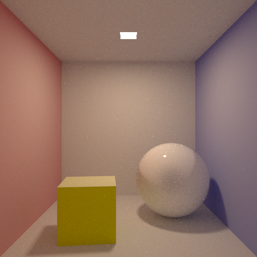
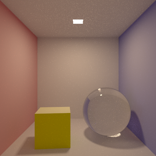
I have successfully added an unbiased direct lighting calculation into the renderer which makes it possible to render more complex scenes with smaller and sparser light sources. Below are two images rendered with direct lighting and a small (1x1) light source simulating a 3400k bulb. In the top image a white ceramic sphere is shown while in the second image it is replaced by a glass one.
50 Samples:
250 Samples: This image was given more time to converge due to the caustics under the glass sphere which converge slower.
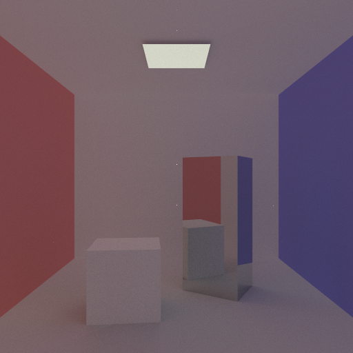
Work on Bi-Directional Path Tracing within the renderer is, sadly, going a lot slower. Currently direct shadows and the more subtle ambient occlusion style effects of global illumination are being washed out of the images. I believe the problem lies with how I am weighting together the contributions from all the different generated paths for a given pair of eye & light subpaths.
As you can see below, only the more dramatic effects of ambient occlusion remain around the bases of the two hemi-cubes. All other detail is lost.
Today has been a pretty good day, both for me and for my work. For the last couple of weeks I’ve been working from home because all I am doing lately is background reading and coding my new renderer. At first it was nice to know that my workspace was only a commando roll (or a fall) out of bed away from me; but after 3 weeks it just got to be a bit much. Don’t take this to mean I didn’t leave the house for three weeks, I did, but working long hours from the comfort of my room did dramatically take its toll on me.
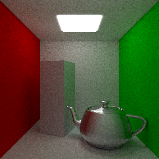
But enough about me going mad in the house! Today I came into the office (which I think I’ll start doing a lot more often) and have made great progress on my new C++ render!