Experiments with Depth-Of-Field

So this evening I thought I’d have a look’see at some of the more advanced ray tracing techniques that I didn’t have time to play with during my dissertation research. Namely, Depth-Of-Field and Specular/Glossy Reflections.

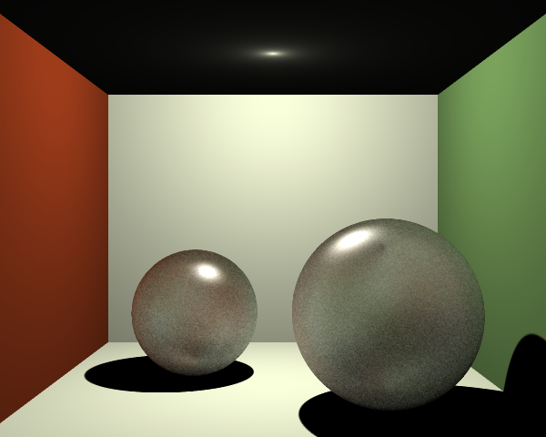
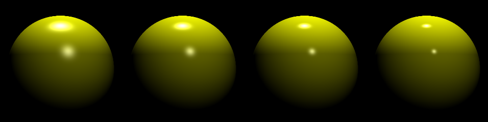
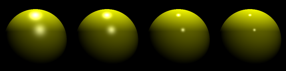
Essentially, Depth-Of-Field mimics the focus point of an eye or camera. Where there is a set focal distance where everything is crisp and in focus, and everything before and after the point becomes progressively more fuzzy as it gets further from that point. To perform DOF on a ray tracer we sample multiple rays for each of our original primary rays, each at a slight offset.

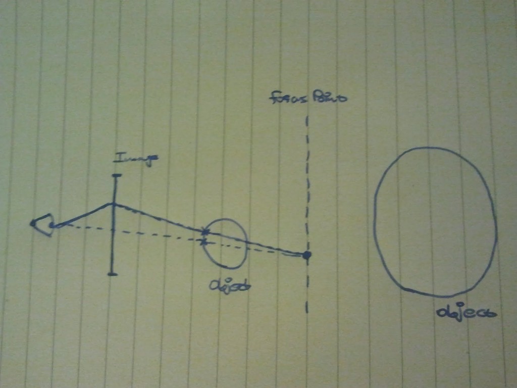
In the image below the dotted line represents the ‘true’ original ray path to the first intersection with a geometry. The solid line represents a sampled ray which has been offset from the origin by a random amount. Both rays pass through the same point in the focal plane which is exactly the focal distance away from both ray origins. Any objects at the focal plane will appear crisp and in focus while anything closer or further will appear out of focus. This can be visualized by the two rays (solid and dotted) intersections with the sphere. Each will return a different colour which when averaged will produce the blurred colour of the out of focus sphere.

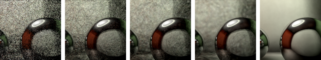
Here is the effect of a 3×3 unit aperture using 25 random samples per ray. As you would expect the render took around 25 times longer to produce the final output, which is worrying because truth be told we really need 100+ samples (closer to 300-500) to produce smooth and clear results without noise.

Here the quality of the DOF simulation has been upped, however I had to turn off photon mapping to accommodate the increased workload. Here we are rendering with a 3×3 unit aperture but at 100 samples per pixel.

I think tomorrow I might look at some of the more efficient ways of computing DOF. There’s a rather neat method with relies on storing the depth that each pixel is in the image and using that to apply a weighted blurring function after the image has been rendered. Cheating I know but it will be a hell of a lot faster than multiplying the entire workload of the render by an incredibly large sample size.

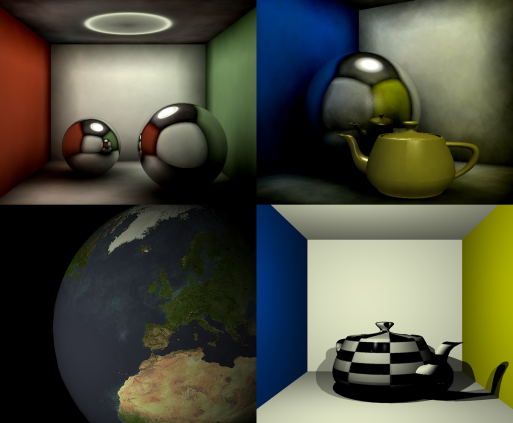
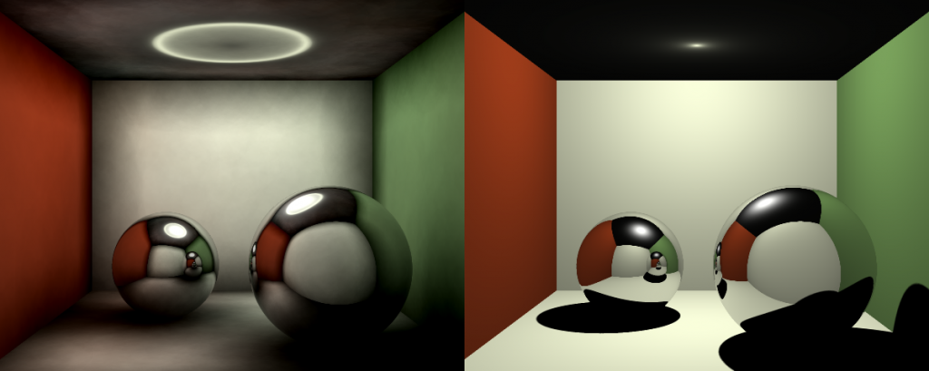
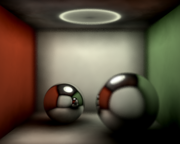
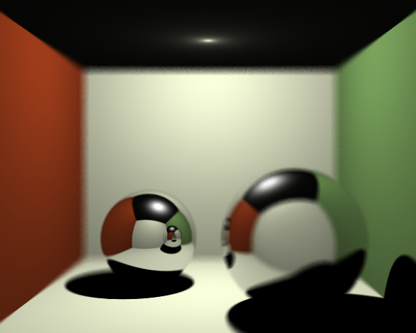
Finally, this evening I had a ‘brief’ (3 and a half hours of reading, coding, swearing, reading, debugging, reading, swearing, crying, and coding) go at trying to implement Glossy Reflections (otherwise known as specular reflections). Well… As you can see in the image below it all works perfectly and it wasn’t a colossal waste of time and energy…. …. …. I’ll try again another time.

Tags Depth of Field, Global Illumination, Ray Tracing

New Java Ray Tracer

As part of the research for my dissertation on GPU Accelerated Path Tracing I thought it would be a good idea to have another crack at writing a Ray Tracer. Unlike my previous ray tracer which was slow, clunky, and produce sub-par results I think this time I’ve done a pretty good job.

The new ray tracer includes a bunch of advanced features such as Texture/Specular/Normal Mapping, Octrees, Photon Mapping, and Adaptive Super-Sampling.

The part of the ray tracer I am most pleased with has got to be Photon Mapping, which is the process of simulating natural and secondary lighting.

Before rendering begins photons are fired out of the light sources in the scene and are bounced around as they collide with objects. At each collision a photon is posed a choice, “Do you die? Or do you keep on living?”, if the photon dies it takes the colour of where it intersected and it is stored in the photon map; on the other hand if the photon decided to live it picks up a little bit of light from its current position and a reflection vector is calculated, it is then fired off in the new direction.

In the image below you can see the effect of Photon Mapping (left) and what the scene would have otherwise looked like without it (right).

An implementation of the K-Nearest Neighbor algorithm was used for searching the photon map for nearest photons to a given intersection location. The algorithm was optimized by storing intermediate photon maps for each object in the scene (triangular meshes were treated as single objects).

The effects of different K values on the K-Nearest Neighbour algorithm can be seen below. The K values used (in order) were: K = 1, K = 10, K = 50, K = 100, K = 500

Lambert shading gives diffuse colour for objects such that the further away they point from a light source the darker they appear.

Phong shading calculates the Specular Highlights that appear on glossy objects. The phong shading is added to the diffuse (lambert) shading to yeild the final colour.

Blinn-Phong shading is an optimization on phong shading which is faster to compute while offering similar results. Phong shading computes specular highlights using an expensive reflection vector calculation; Blinn-Phong shading improves on this by computing a half-way vector between the view direction and the light source to use for estimating the specularity of the surface.

Tags Global Illumination, Photon Mapping, Ray Tracing