A 3D Printed case for my Raspberry Pi
May 6, 2014 - 11:38 pm by Joss Whittle 3D Printing L2Program Raspberry Pi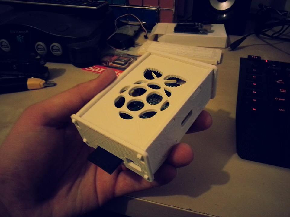
Just a simple 3D Printed Case for my Raspberry Pi. :)

Just a simple 3D Printed Case for my Raspberry Pi. :)
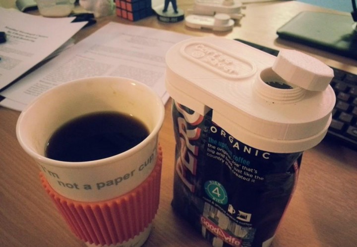
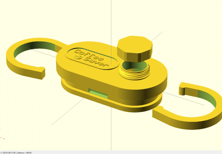
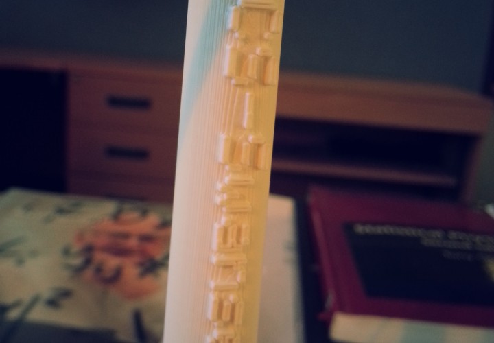
Coffee Saver is a project to create a reusable and versatile cap for an open bag of coffee granules, which can be produced on a 3D Printer.
Find this project on Thingiverse or on Github!
The main CAD software used for this project is OpenSCAD with additional functionality provided by Dan Kirshner’s OpenSCAD Threading Library and PGreenland’s Text Library.
Before I found out I’d be doing a PhD this year I submitted an MEng project proposal to a professor in my department with the idea to build a cheap 3D Printer out of Lego Technic. The plan was to use the ready available, and easy to assemble parts and motors of the Lego Technic along side a powerful yet easy to program Arduino unit is a brain. I even got so far as to make some preliminary CAD mockups and a working mockup of the chasis.
But with starting my PhD research, I was forced to shelve the project (like so many others) so as to focus on my actual work.
Lately however, it came to my attention that the Computer Science department had bought a Makerbot Replicator 2X 3D Printer which is available to members of the research group as both a research tool, and as a teaching tool. The mumbling consensus in the department is that it’s fine to use the printer “within good reason and common sense…”, and that the logic of “teaching yourself to use it means you can potentially teach undergrads about it in the future…” means that as long as it doesn’t hinder us or other peoples research it’s fair to use it!
After all, what’s the point in owning the fun toys if we don’t play with them? :)
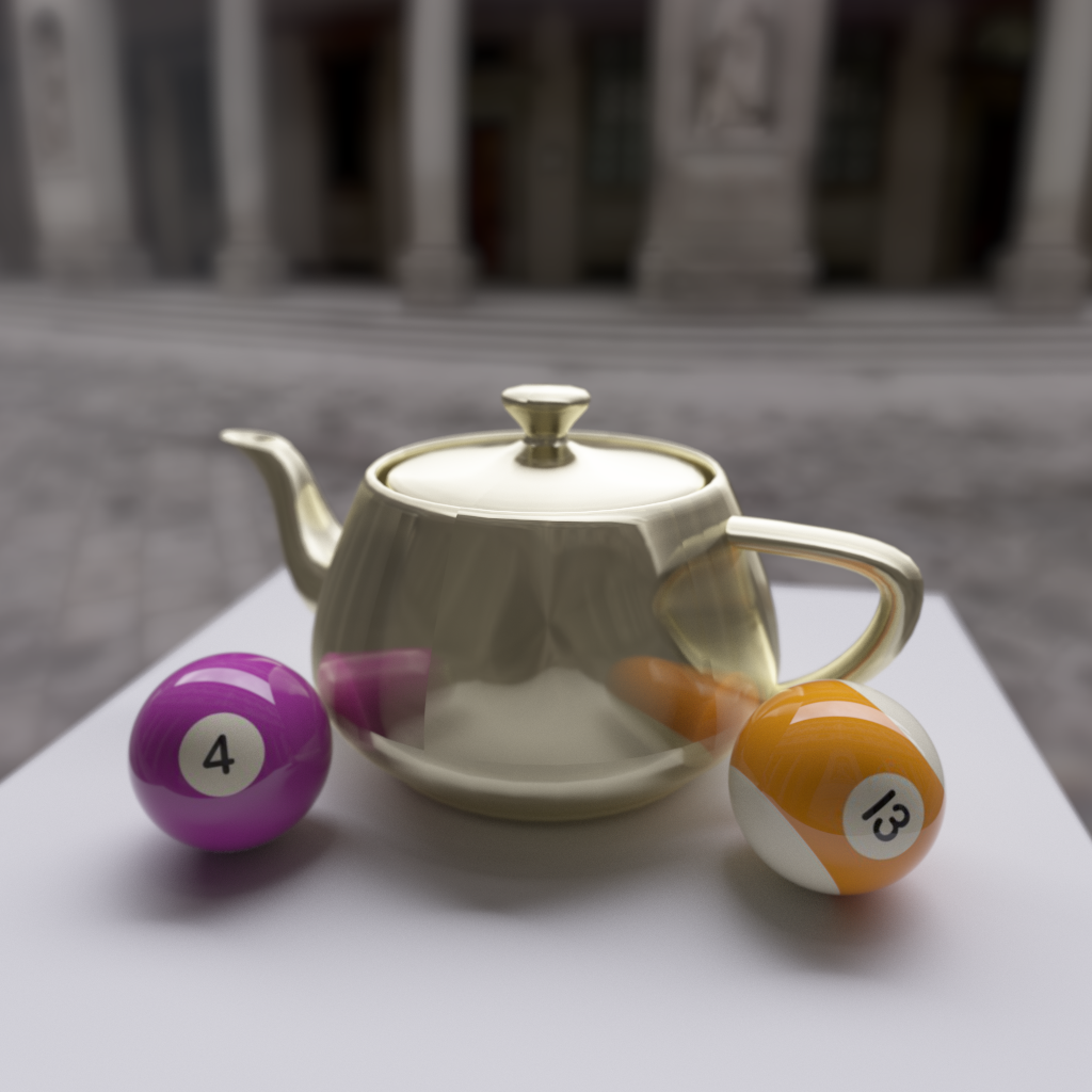
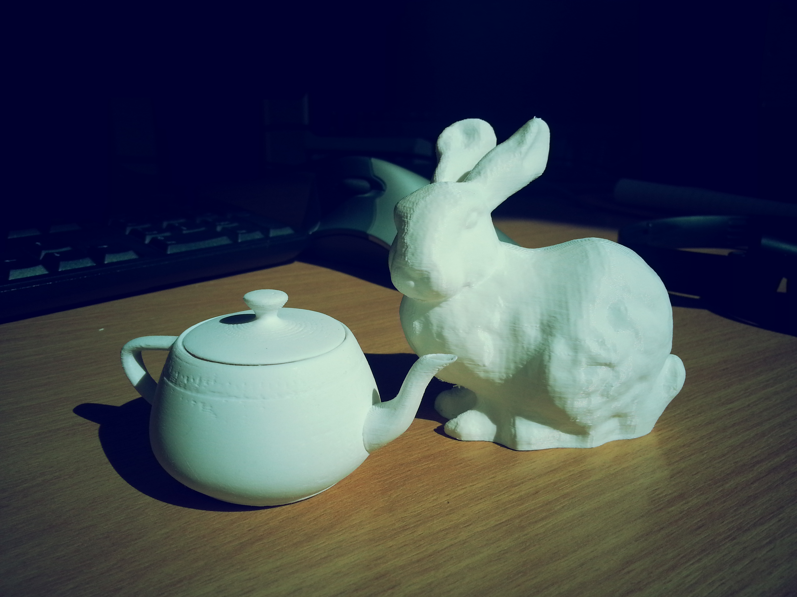
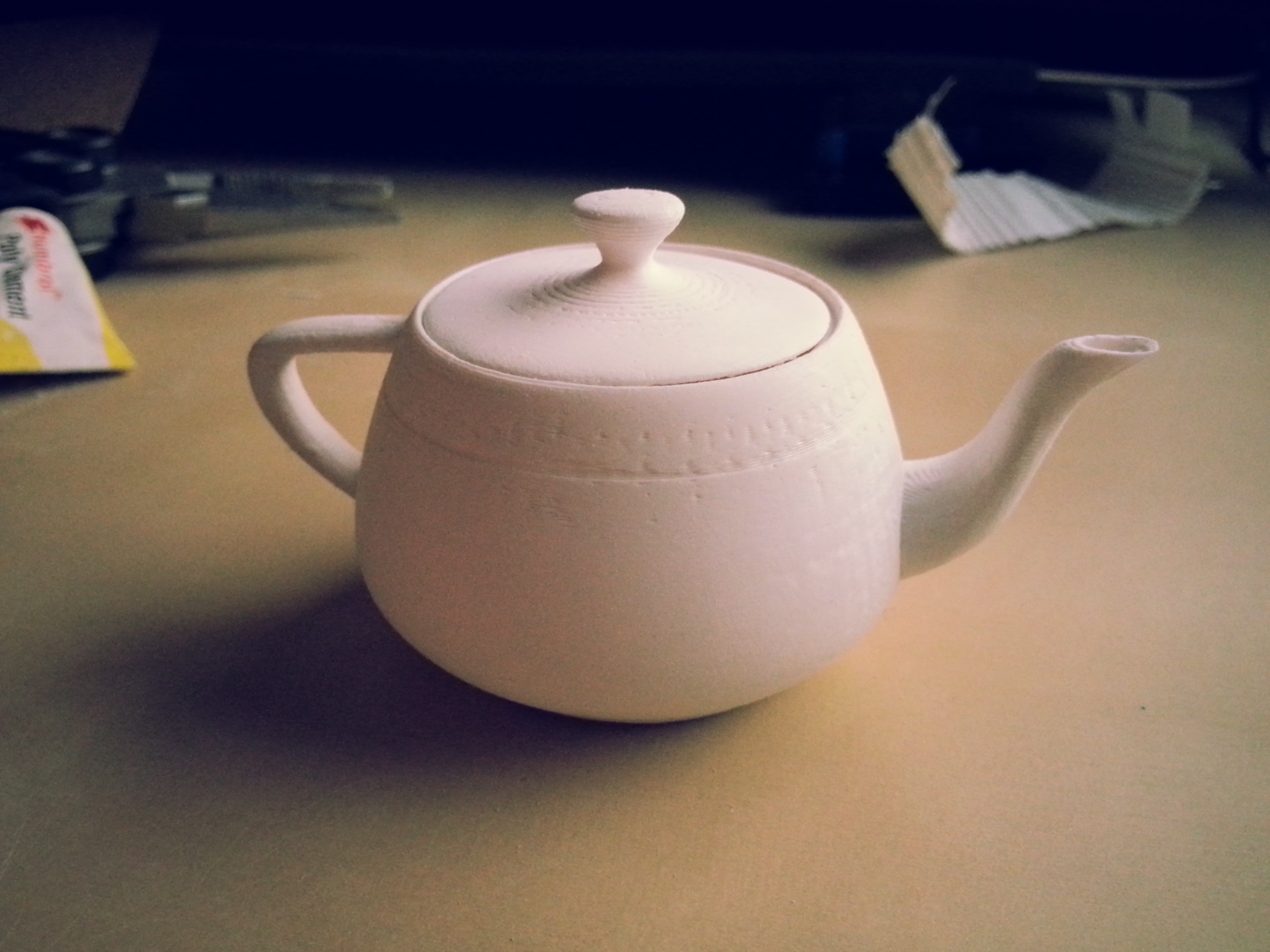
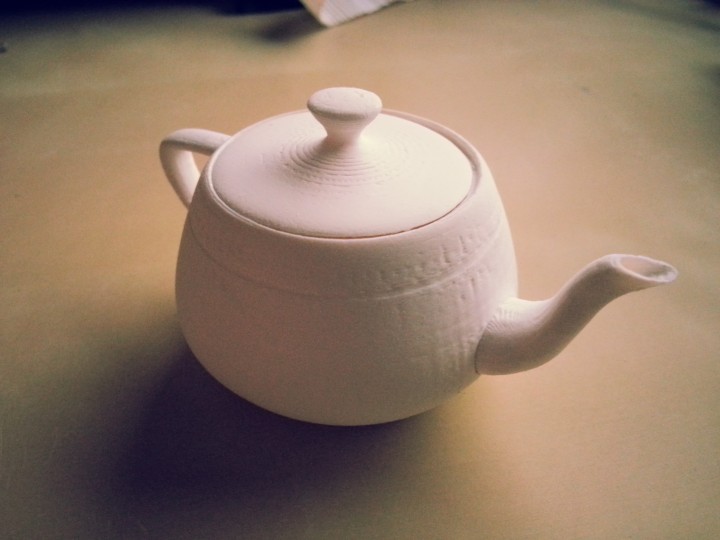
With this in mind there’s been something on my list of Stuff I want to own: for a long time, that is of course a Utah Teapot!
The Utah Teapot is a famous dataset in the Computer Graphics community and used to be an official measurement of graphics performance in terms of Number of Teapots rendered / Second (I’m not kidding).
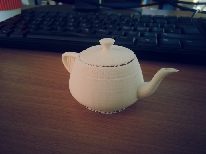
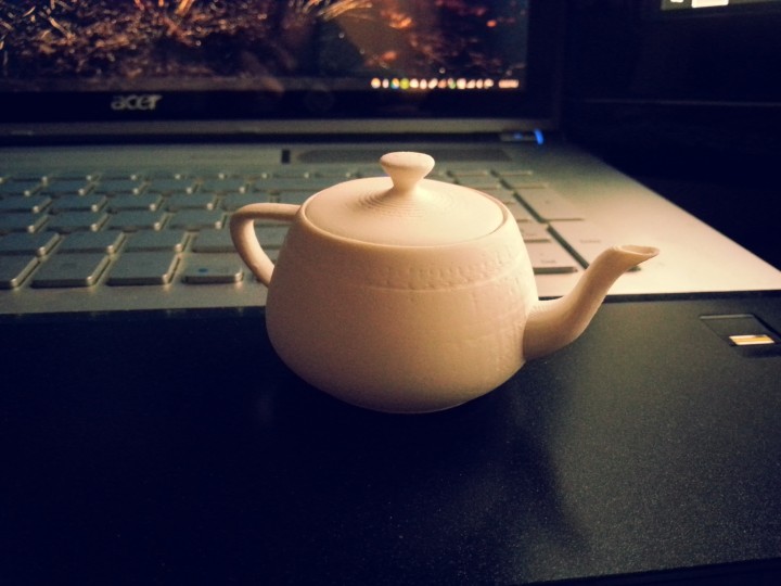
After a few hours of playing around modifying the original dataset in Autodesk Maya to flesh it out as a proper object it was time to print! Yes I know, I almost certainly could have found a better model online that was properly modified and tested on a 3D Printer.. but this is a dataset I have been rendering and working with for years now and it only felt right that I should try to modify it myself to print one. Though if I ever go back to print another teapot, bigger, I’ll definitely be using one like I linked that was designed in AutoCAD rather than an Artistic Modelling package.
The whole print took just over 100 minutes to complete, and I probably spent an additional ~30 minutes or so sanding it down with some fine grit sandpaper to give it a smooth finish.
Pressing onwards with research after a short break to play with the Xeon Phi rack, I’ve been working on visualizations for Monte Carlo Simulations.
My aim is to have a clean and concise means of displaying (and therefore being able to infer relationships from) the data of higher dimensional probability distributions. The video below shows one such visualization where a 2D Gaussian PDF has been simulated using Hamiltonian Dynamics.
The two 3D meshes represent the reconstructed sample volume as a 2D histogram of values rescaled to the original function. The error between the reconstruction and the original curves is shown through the colour of the surface where hot spots denote areas of high error.
The mean sq error for the whole distribution is displayed in the top right on a logarithmic scale. An algorithm which converges in an ideal manner will graph it’s error as a straight line on the log scale.
The sample X and Y graphs in the bottom right allow us to visualize where the samples are being chosen as the simulation runs and infer about whether samples are being chosen independently of one another. The centre-bottom graph simply gives us a trajectory of samples over the course of the simulation. This allows us to additionally catch if an algorithm is prone to getting stuck in local maxima’s.
The above video shows the same simulation run with a basic Metropolis Hastings algorithm. Here the proposal sample x and y attributes are chosen independently of one another, meaning this is not a Gibbs Sampler. Although I intend to implement one within the test framework for comparisons sake soon.
A key difference between the two simulations here is to note the Path Space Trajectory shown in the bottom-centre graph and how it relates to the Sample Dimension Space graphs shown on the middle & bottom-right. Hamiltonian Dynamics chooses sets of variables where the x and y elements are highly dependent on one another within a coordinate, yet almost entirely independent of other pairs of coordinates within the Path Space.
Metropolis Hastings on the other hand, chooses coordinate pairs entirely independently of one another, and values within each dimension of the Path Space that are highly dependent on one another. These characteristics of the Metropolis sampler are undesirable, which is why adding a dependency within coordinate pairs (Gibbs Sampling) helps to accelerate multi-dimensional Metropolis Samplers.
It’s been a couple of weeks since I stopped working directly on rendering and took some time to read up on a topic called Hamiltonian (Hybrid) Monte Carlo which is to be the main focus of my research for the foreseeable future.
Hamiltonian Monte Carlo comes from a physics term of the same genesis called Hamiltonian Dynamics. The general idea being that, like with a Lagrangian equation for a system, you find a way to model the energy of a system which allows you to estimate it at efficiently even when the system is highly dimensional. With a Lagrangian you aim to minimize the degrees of freedom to reduce computation, and similarly with a Hamiltonian you reduce the problem to a measure of the systems kinetic K(p) and potential U(x) energy. This allows you to describe the entire state of an arbitrarily dimensional system as the sum of these measures, i.e. H(x,p) = U(x) + K(p)
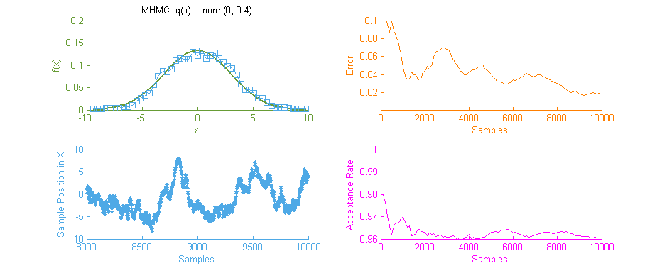
Above is our faithful companion, Metropolis Hastings Monte Carlo (MHMC), simulating a Normal distribution with mean “ and variance 3. The simulation was run for 10,000 samples yielding the shown results. Some things worth noting here are features such as the Error curve (Orange), which varies dramatically as simulation progresses. This is in-part due to the nature of the Random Walk which MHMC takes through the integration space which can be seen in the Blue graph to the bottom left. It is clear from the Blue graph that two states x and x' in the Makrov Chain are tightly dependent on one another.
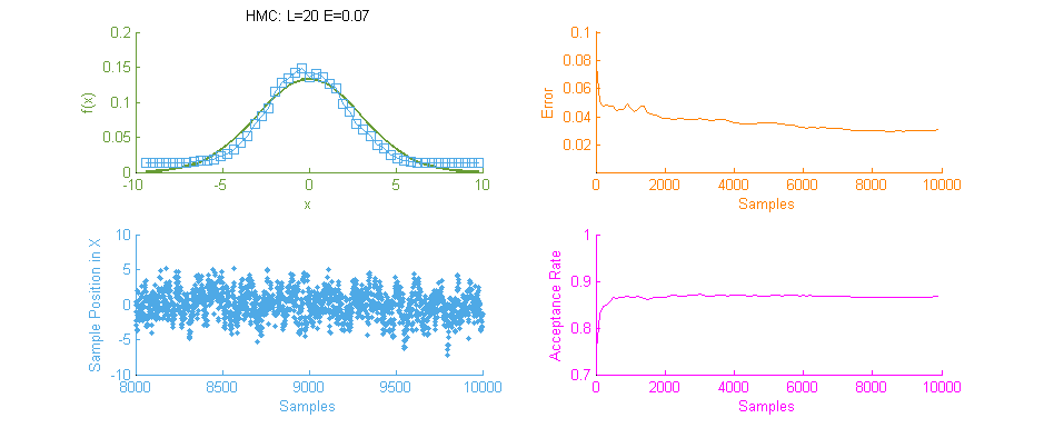
Next we see the same Normal distribution used above, estimated this time using Hamiltonian Monte Carlo (HMC) with trajectory length 20 and step size 0.07. To compare this to our previous simulation using MHMC several things become apparent. Firstly, The Error curve (Orange) seems to decay in a much more controlled and systematic manner. As opposed to the Error for MHMC which was erratic due to the nature of a Random Walk, here we see the benefit of making an informed choice as to where to place the next sample. From this we can hypothesise that a optimally tuned HMC simulation will in general reduce the error of the simulation with more samples consistently with little chance of introducing large, random, errors as with MHMC. Additionally in the sample placement graph (Blue) we see that the relationship between two states x and x' is far more abstracted, meaning two samples while being related and forming a valid Markov Chain will not reduce the accuracy of the simulation by treading on each others turf.
There is however, an issue with the above HMC simulation. Tuning. Unless properly tuned for the specific problem the Hyper-parameters for the Trajectory length L and Step size E will simply not work as intended and will yield poor results.
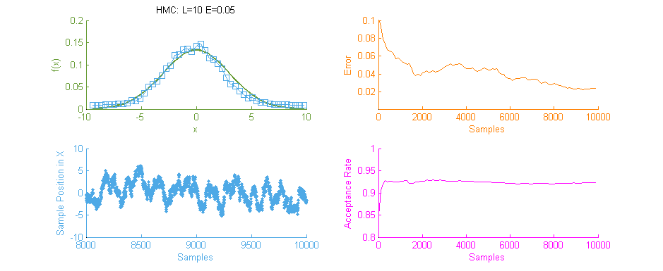
Above is a second run of the HMC simulation, this time with trajectory length 10 and step size 0.05. Because the length of the Leapfrog Trajectory was not sufficient to allow the system to move to an independent state we see the same banding of samples in the sample frequency graph (Blue) as we saw in the original Metropolis simulation. Additionally because of the dependent nature of the samples a similar pattern is seen in the Error curve (Orange) where the curve has large peaks where error was reintroduced to the system like with a Random Walk.
It is therefore vital to optimally tune HMC as the computation for each sample is an order of magnitude larger than with MHMC. Without proper tuning it’s much better to stick with the easier to tune MHMC.