Direct Lighting cont.

Continuing on with my work implementing direct lighting contributions to the renderer I thought I’d take a second to show off some shots I’m most happy with.

This first shot I am most pleased with, though it could possibly be subject bias due to my having stared at it for hours as I program; however, I am convinced this looks physically plausible. Or at least, it’s the most physically plausible thing I have rendered so far. This image was rendered using 1250 samples with a 1 unit thick coat of clear varnish on the diffuse red sphere.

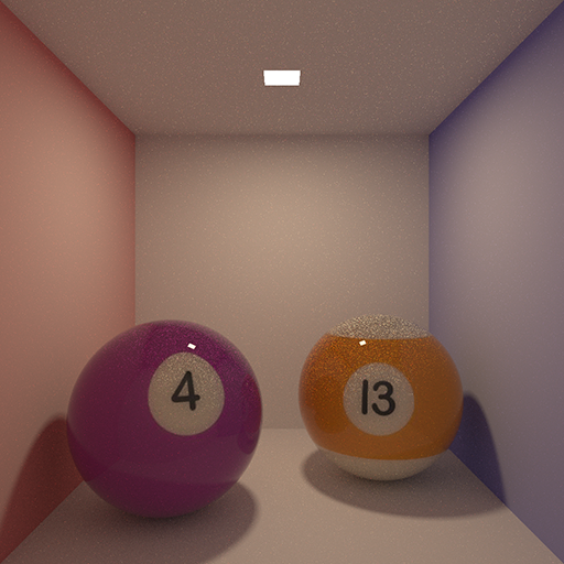
I decided to try combining the sphere shader with texture mapping to see how good it would look as a glossy stone shader. Due to the high variance from the two balls this image was rendered at 2x resolution (1024 x 1024) and then downsized back to the normal resolution. The upscaled image was rendered with 100 samples.

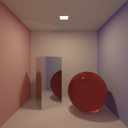
The next image was rendered using 1000 samples. Despite the increased convergence speed of the red glass sphere compared to the ceramic one in the first image, the presence of mirror box adds variance back into the image due to it’s broad specular caustics.

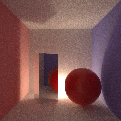
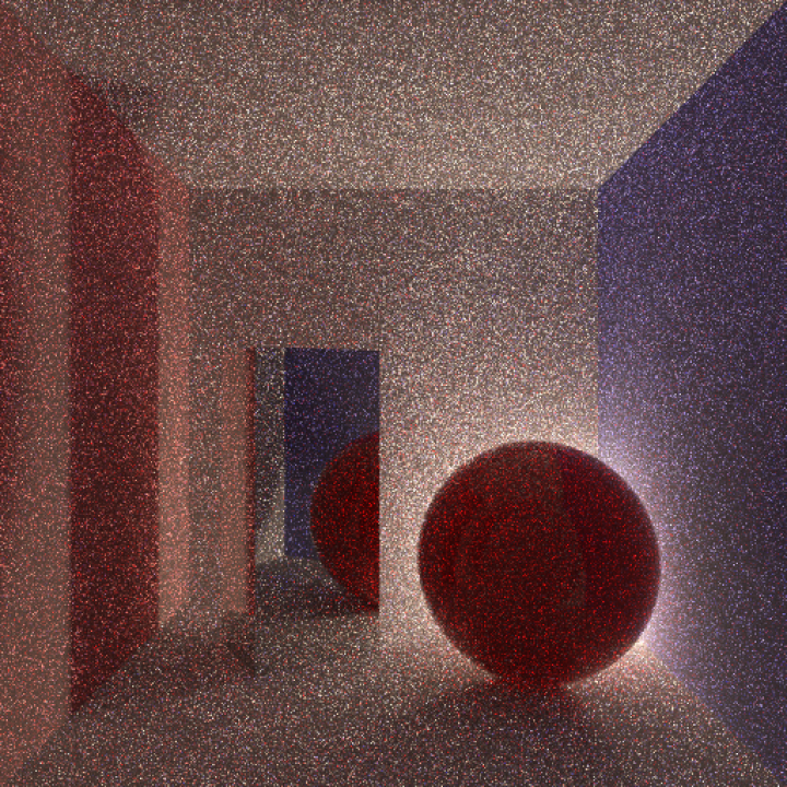
I also experimented with testing different light positions to see how robust the direct lighting contribution was compared to Naive Path Tracing alone. A more complete comparison of light positions using 25 samples per image is shown further down this post. For the next image, the light is placed on the floor along the rear wall of the Cornell Box. The shot was rendered with 1000 samples and 1 unit varnish on the sphere.

Next the same shot is shown, this time rendered with only 250 samples and a clear glass sphere. Even after this relatively small number of samples, well defined caustics can be seen on the right wall and on the surface of the sphere, indirectly, through the mirror box.

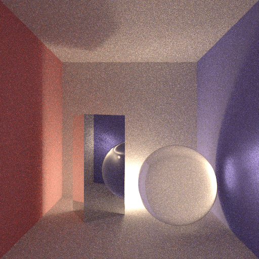
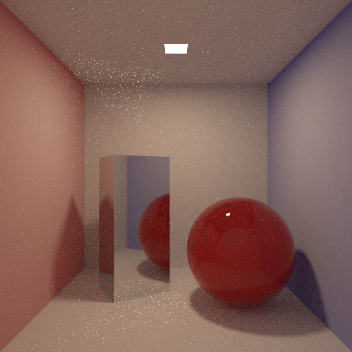
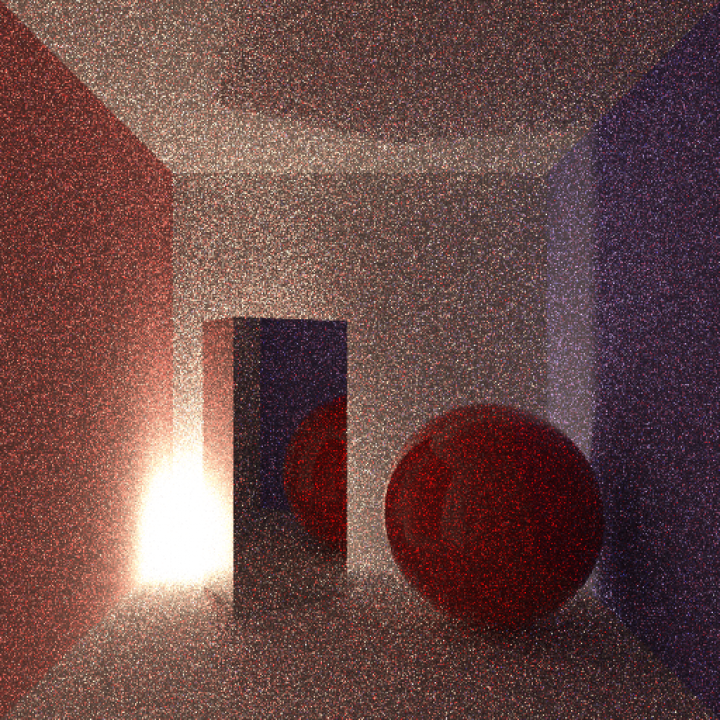
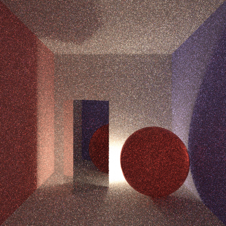
Light connectivity comparison: (25 samples each)

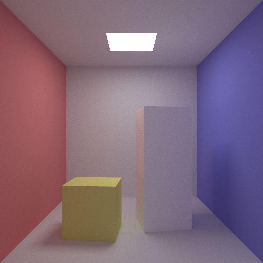
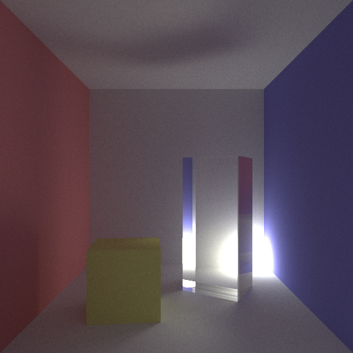
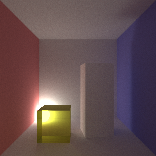
Below, four renders are shown with varying light positions. The overhead light is a 1 x 1 unit square which emits light uniformly in a downward facing hemisphere, while the three backlit images are lit by unit spheres placed just above the ground.

As you can see, while convergence is still impressive for such a low sample count using a small surface area light source, variance still remains a major issue. Now that I know the direct lighting calculation works however, I think it can be implemented into the Bi-Directional Path Tracer which should help solve some of it’s shading issues.

Tags Global Illumination, Monte Carlo Integration, Path Tracing, Ray Tracing

Direct Lighting for (not so) Naive Path Tracing

Finally starting to make up for the time I took off over christmas!

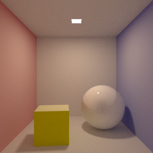
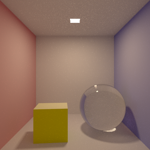
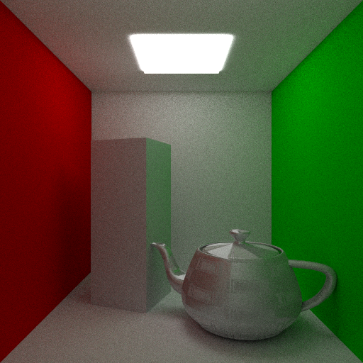
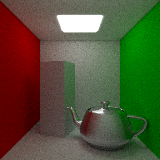
I have successfully added an unbiased direct lighting calculation into the renderer which makes it possible to render more complex scenes with smaller and sparser light sources. Below are two images rendered with direct lighting and a small (1x1) light source simulating a 3400k bulb. In the top image a white ceramic sphere is shown while in the second image it is replaced by a glass one.

50 Samples:

250 Samples: This image was given more time to converge due to the caustics under the glass sphere which converge slower.

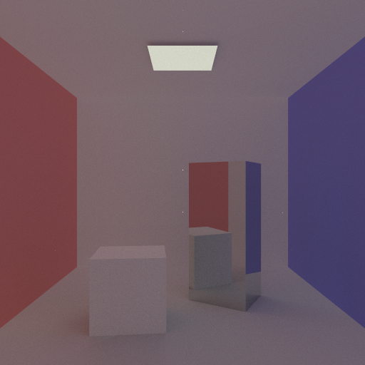
Work on Bi-Directional Path Tracing within the renderer is, sadly, going a lot slower. Currently direct shadows and the more subtle ambient occlusion style effects of global illumination are being washed out of the images. I believe the problem lies with how I am weighting together the contributions from all the different generated paths for a given pair of eye & light subpaths.

As you can see below, only the more dramatic effects of ambient occlusion remain around the bases of the two hemi-cubes. All other detail is lost.

Tags Bi-Directional Path Tracing, Global Illumination, Monte Carlo Integration, Path Tracing, Ray Tracing

Some more test images

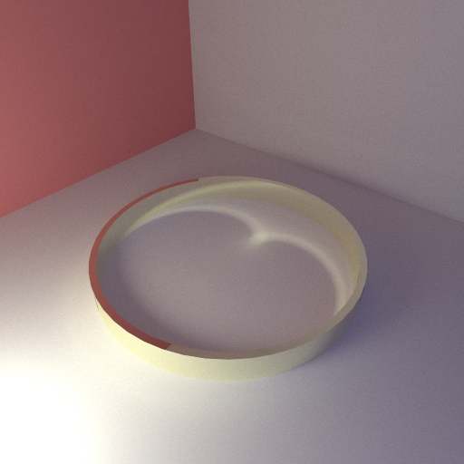
Thought it was about time to test some caustics on the renderer. Lately I’ve been both fascinated and frustrated by the strange forms and shapes that occur when light refracts and reflects off of lit surfaces. A great example of this is a metallic ring laying on a diffuse surface. Light bouncing onto the inside edge of the ring will be focused downwards onto the floor plane in a curved m shape causing a bright spot.

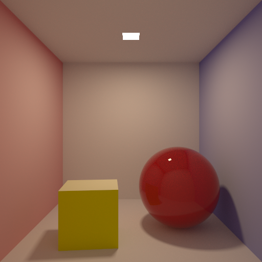
I’ve also been playing around with scenes that employ more indirect lighting. By this I mean scenes where the light source(s) are mostly if not entirely occluded from direct view by the camera. To this effect I set a standard cornell box scene with a yellow cube and a white oblong inspired by Cohen & Greenberg,and placed an occluded light sphere in the back-bottom corner of the room. I then toggled which of the two hemicubes were made of glass to see how the light would refract through them.

Tags Global Illumination, Monte Carlo Integration, Path Tracing

Refraction and an Unbiased (read “fixed”) lighting model

Tags Global Illumination, Monte Carlo Integration, Path Tracing

BRDF Comparison

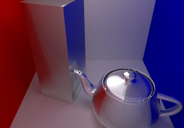
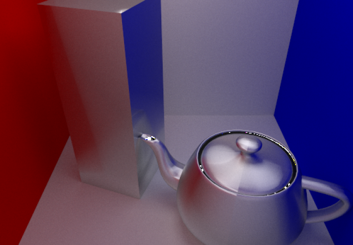
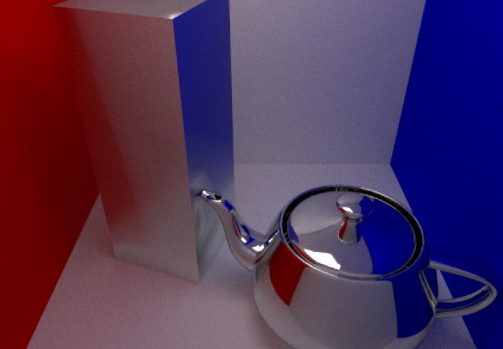
I thought I’d make some high quality comparison shots of some of the shaders I’ve been working on. Above you can see a side by side comparison of a perfect mirror BRDF and a Phong based BRDF with exponents of one million and ten for the centre and right images respectively.

While the Phong-like BRDF does give nice glossy reflections at a relatively small cost it does not model a physically accurate shader. I’m currently looking into implementing a Cook–Torrance model shader which while being more time consuming to compute gives nice results which are based off of physical phenomena. The Cook–Torrance shader also has the inherent ability to model microfacets within the surface of objects which is a big plus.

Because the Phong BRDF is not physically accurate I needed to find a PDF that would look correct in the renderings. The Mirror BRDF for instance has a PDF = 1 and the Diffuse BRDF has a PDF = 2 * (normal . newDirection). After some experimenting from reading a paper that claimed the Phong marginal pdf was cos(theta)^e which I understood (possibly incorrectly as it did not work) to mean PDF = (normal . newDirection)^e I found (gave up) that the Diffuse BRDF in fact worked reasonably well for the Phong model.

Edit I have found a better paper with what looks like a good Phong model. They even give a run down of using their model in a Monte Carlo style simulation with a marginal PDF. I might try implementing this before I move onto Cook-Torrance.

Tags Global Illumination, Monte Carlo Integration, Path Tracing

Tree visualization and specular mapping

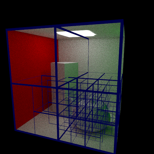
Previously I’ve debugged my KD-trees only by looking at archaic console printouts where at best each descending node in the structure is tabbed a couple of spaces further in from it’s parent.

However, seeing as I’m currently building a new renderer it seemed apt to build in a method for visualizing the generated trees. This was pretty simple to add in, if a preprocessor flag __AABB_EDGE__ is defined at compile time then during tree traversal additional code will run which does a simple UV coordinate calculation for the Axis Aligned-Bounding Box; if the UV is close enough to the edge of the box then the current pixel is abandoned and set to plain blue. The result is quite interesting to view and because of the power of the C++ preprocessor when it is disabled it effectively doesn’t exist in the compiled executable, meaning it has no effect on performance.

I have also been playing with specular and normal mapping. It was trivial to add due to the design of the shader class this time. In the case of specular mapping the max value of each RGB tuple is taken as the value for the map on the [0,1] range; this is then used to linearly scale the specular exponent of the shader which is used to calculate the glossy reflection for surfaces with an exponent > 0. Below a checker-board texture was used to scale a specular exponent of 128 into regions of 0 and 128 over the surface of the teapot.

Tags Global Illumination, Monte Carlo Integration, Path Tracing

Feels good to be back in the office

Today has been a pretty good day, both for me and for my work. For the last couple of weeks I’ve been working from home because all I am doing lately is background reading and coding my new renderer. At first it was nice to know that my workspace was only a commando roll (or a fall) out of bed away from me; but after 3 weeks it just got to be a bit much. Don’t take this to mean I didn’t leave the house for three weeks, I did, but working long hours from the comfort of my room did dramatically take its toll on me.

But enough about me going mad in the house! Today I came into the office (which I think I’ll start doing a lot more often) and have made great progress on my new C++ render!

Tags Concurrency, Global Illumination, Monte Carlo Integration, Path Tracing, Ray Tracing

More pretty graphs…

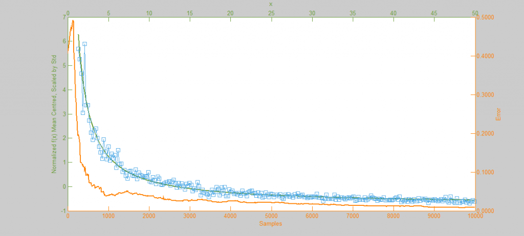
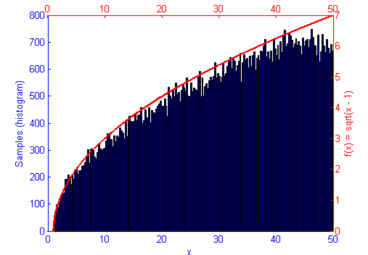
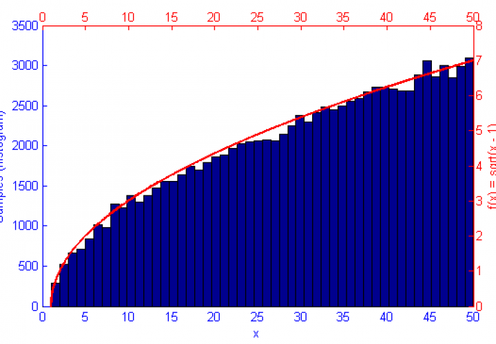
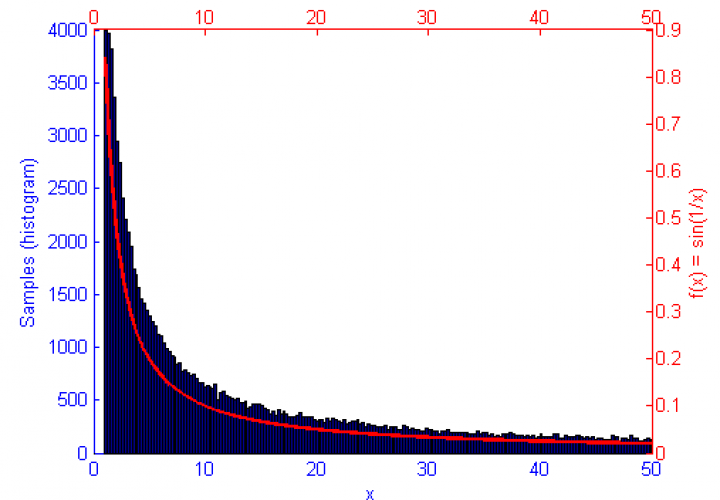
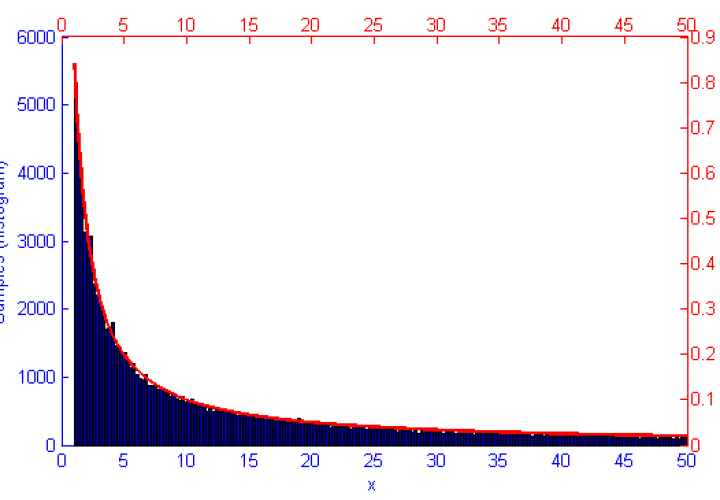
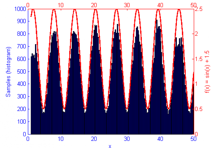
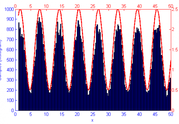
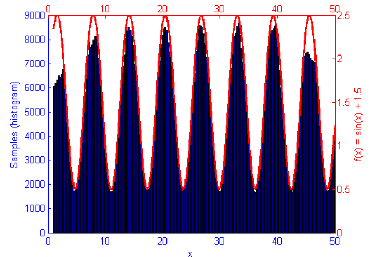
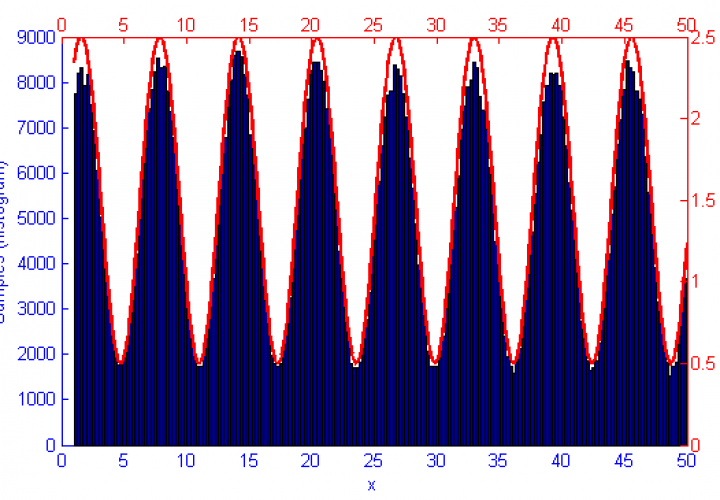
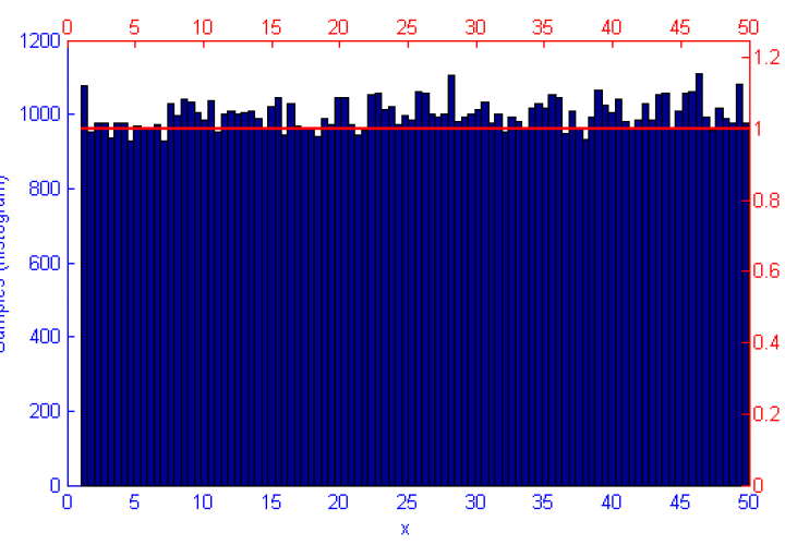
So I’m still playing with graphs in Matlab… I shouldn’t complain, I know. I should be cherishing how laid back and relaxed the PhD experience is right now compared the where I’ll be a couple of years from now.

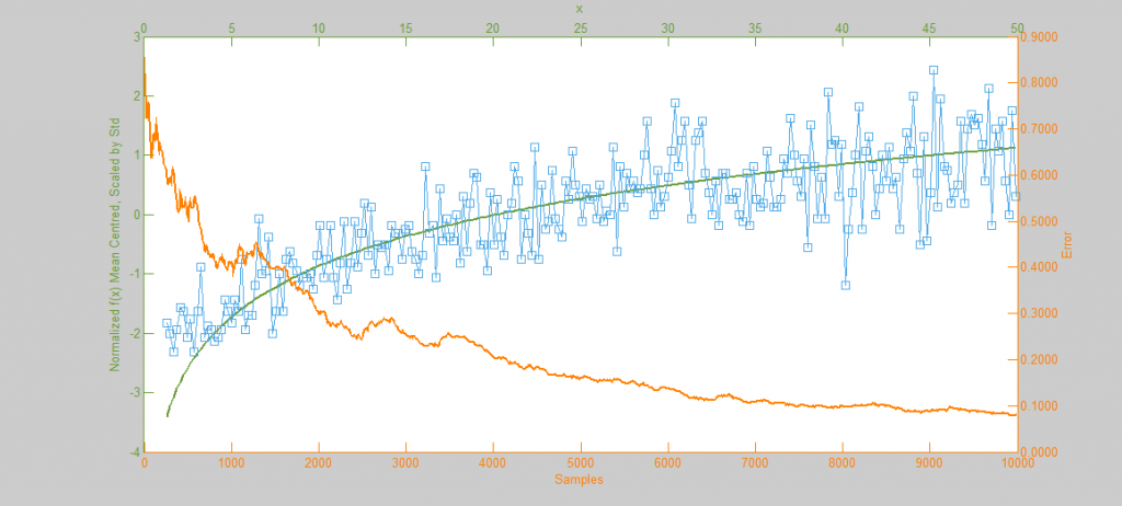
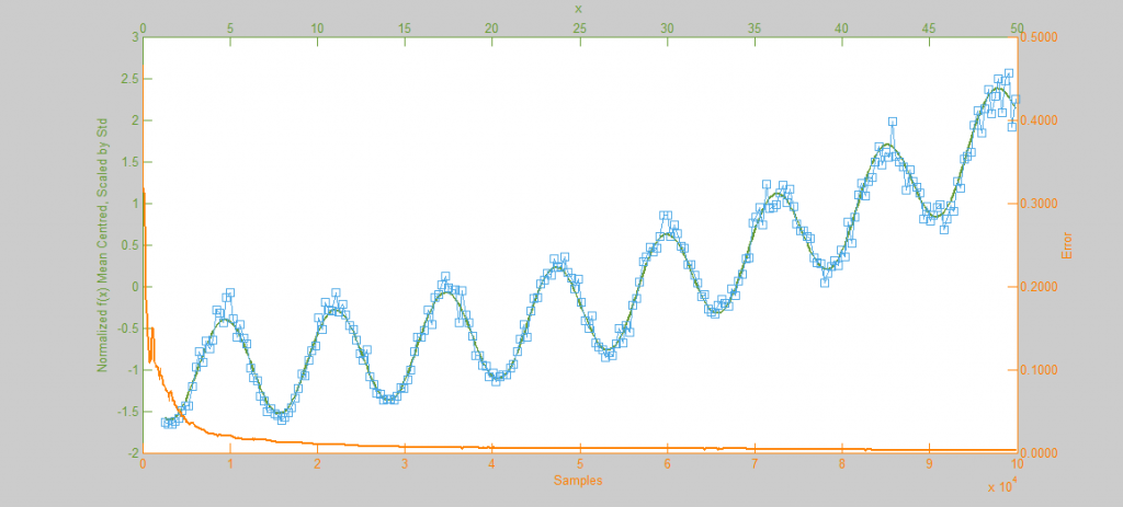
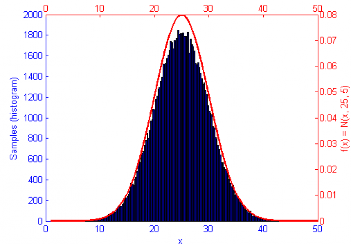
The function f(x) is shown in green, the sample distribution in blue with histogram bins marked as circles, and the error curve in orange. Since creating these images I’ve begun drawing the error on the log x log scale which displays as a linear decay as you’d expect.

Tags Accept-Reject, Metropolis-Hastings, Monte Carlo Integration

More Bi-Directional Path Tracing

It’s still not perfect, far from it in fact, but it’s progress none the less. I’ve been reading a lot lately about Metropolis Light Transport, Manifold Exploration, Multiple Importance Sampling (they do love their M names) and it’s high time I started implementing some of them myself.

So it’s with great sadness that I am retiring my PRT project which began over a year ago, all the way back at the start of my dissertation. PRT is written in Java, for simplicity, and was designed in such a way that as I read new papers about more and more complex rendering techniques I could easily drop in a new class, add a call to the render loop, or even replace the main renderer all together with an alternative algorithm which still called upon the original framework.

I added many features over time from Ray Tracing, Photon Mapping, Phong and Blinn-Phong shading, DOF, Refraction, Glossy Surfaces, Texture Mapping, Spacial Trees, Meshes, Ambient-Occlusion, Area Lighting, Anti-Aliasing, Jitter Sampling, Adaptive Super-Sampling, Parallelization via both multi-threading and using the gpu with OpenCL, Path Tracing, all the way up top Bi-Directional Path Tracing.

But the time has taken it’s toll and too much has been added on top of what began as a very simple ray tracer. It’s time to start anew.

My plans for the new renderer is to build it entirely in C++ with the ability to easily add plugins over time like the original. Working in C++ gives a nice benefit that as time goes by I can choose to dedicate some parts of the code to the GPU via CUDA or OpenCL without too much overhead or hassle. For now though the plan is to rebuild the optimized maths library and get a generic framework for a render in place. Functioning renderers will then be built on top of the framework each implementing different feature sets and algorithms.

Tags Bi-Directional Path Tracing, Concurrency, CUDA, Depth of Field, Global Illumination, GPGPU, Monte Carlo Integration, OpenCL, Path Tracing, Photon Mapping, Ray Tracing

Accept-Reject Sampling

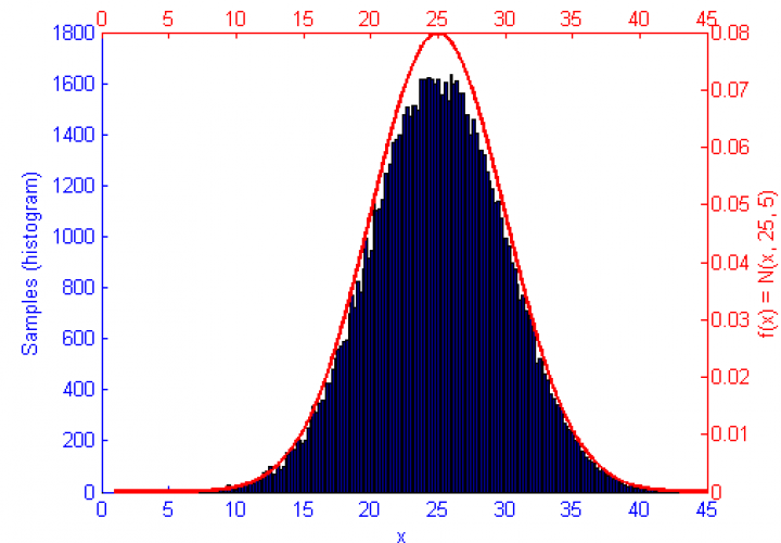
Continuing on from experiments last week with Metropolis Hastings sampling for probability distributions I decided to implement Accept-Reject sampling. Accept-Reject seems to deliver well distributed results faster than Metropolis Hastings does but in the long run can easily introduce biased samples if the proposal distribution q(x) is not well tuned to the specific probability distribution function. MH on the other hand, is far more resilient to an improperly chosen proposal distribution as it will still converge to an unbiased result in most cases, albeit by taking a longer time to converge than it normally would. Accept-Reject also seems to have issues towards the truncations of it’s function causing under-sampling of values close to the lower and upper bounds.

Tags Accept-Reject, Bayesian Statistics, Matlab, Metropolis-Hastings, Monte Carlo Integration